Computational Methods
for GPs
Lecture 23
GPs and Computational Complexity
The problem with GPs
Unless you are lucky (or clever), Gaussian process models are difficult to scale to large problems. For a Gaussian process \(\underset{n \times 1}{\boldsymbol{y}} \sim \mathcal{N}(\boldsymbol{\mu},\boldsymbol{\Sigma})\):
Want to sample \(\boldsymbol{y}\)? \[ \boldsymbol{\mu} + \color{red}{\text{Chol}(\boldsymbol{\Sigma})} \times \boldsymbol{Z} \text{ with } Z_i \sim \mathcal{N}(0,1) \qquad \qquad \color{red}{\mathcal{O}\left({n^3}\right)} \]
Evaluate the (log) likelihood? \[ -\frac{1}{2} \log {\color{red}{|\Sigma|}} - \frac{1}{2} (\boldsymbol{x}-\boldsymbol{\mu})'\; \color{red}{\boldsymbol{\Sigma}^{-1}} \; (\boldsymbol{x}-\boldsymbol{\mu}) - \frac{n}{2}\log 2\pi \qquad \qquad \color{red}{\mathcal{O}\left(n^3\right)} \]
Update covariance parameter? \[ \color{orange}{\{\Sigma\}_{ij}} = \sigma^2 \exp(-\{d\}_{ij}\phi) + \sigma^2_n \, 1_{i=j} \qquad \qquad \color{orange}{\mathcal{O}\left(n^2\right)} \]
A simple guide to computational complexity
\(\mathcal{O}\left(n\right)\) - Linear complexity
Go for it!
\(\color{orange}{\mathcal{O}\left(n^2\right)}\) - Quadratic complexity
Pray
\(\color{red}{\mathcal{O}\left(n^3\right)}\) - Cubic complexity
Give up
How bad is the problem?
Practice - Migratory Model Prediction
After fitting the GP need to sample from the posterior predictive distribution at \(\sim3000\) locations \[ \boldsymbol{y}_{p} \sim \mathcal{N}\left(\mu_p + \Sigma_{po} \Sigma_o^{-1}(y_o - \mu_o) ,~ \Sigma_p - \Sigma_{po} \Sigma_{o}^{-1} \Sigma_{op}\right) \]
| Step | CPU (secs) |
|---|---|
| 1. Calc \(\Sigma_p\), \(\Sigma_{po}\), \(\Sigma_{o}\) | 1.080 |
| 2. Calc \(\text{chol}(\Sigma_p - \Sigma_{po} \Sigma_{o}^{-1} \Sigma_{op})\) | 0.467 |
| 3. Calc \(\mu_{p|o} + \text{chol}(\Sigma_{p|o}) \times Z\) | 0.049 |
| 4. Calc Allele Prob | 0.129 |
| Total | 1.732 |
Total run time for 1000 posterior predictive draws:
- CPU (28.9 min)
A bigger hammer?
| Step | CPU (secs) | CPU+GPU (secs) | Rel. Perf |
|---|---|---|---|
| 1. Calc. \(\Sigma_p\), \(\Sigma_{po}\), \(\Sigma_{p}\) | 1.080 | 0.046 | 23.0 |
| 2. Calc. \(\text{chol}(\Sigma_p - \Sigma_{po} \Sigma_{o}^{-1} \Sigma_{op})\) | 0.467 | 0.208 | 2.3 |
| 3. Calc. \(\mu_{p|o} + \text{chol}(\Sigma_{p|o}) \times Z\) | 0.049 | 0.052 | 0.9 |
| 4. Calc. Allele Prob | 0.129 | 0.127 | 1.0 |
| Total | 1.732 | 0.465 | 3.7 |
Total run time for 1000 posterior predictive draws:
- CPU (28.9 min)
- CPU+GPU (7.8 min)
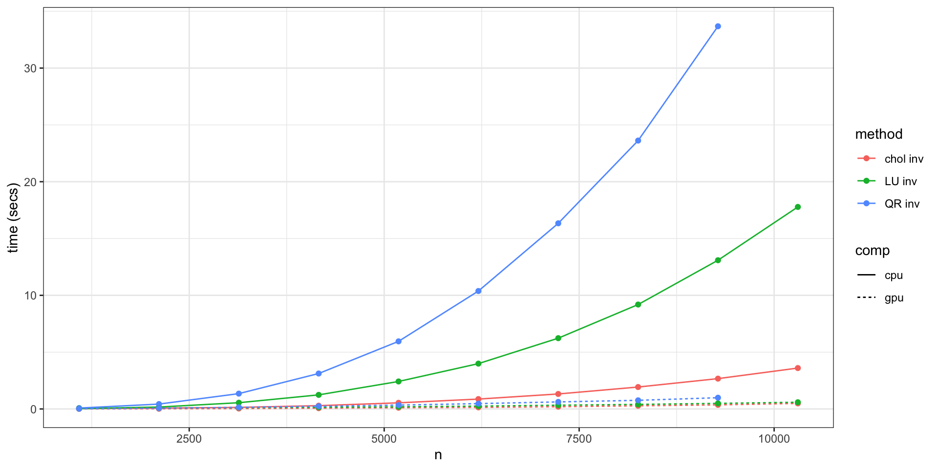
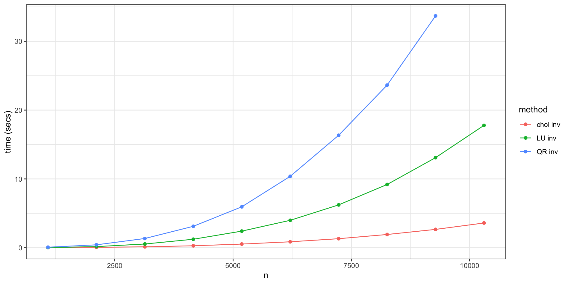
Cholesky CPU vs GPU (P100)

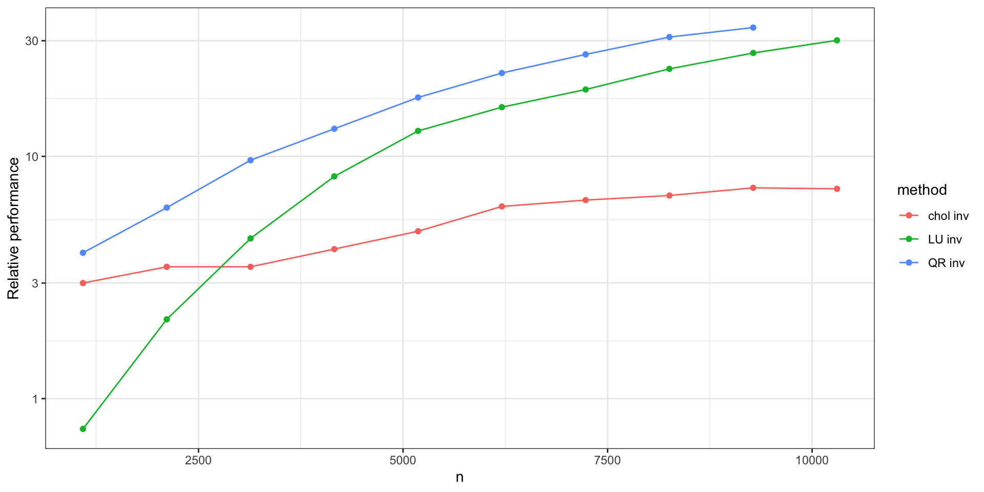
Relative Performance
Aside (1) - Matrix Multiplication (P100)


Aside (2) - Memory Limitations
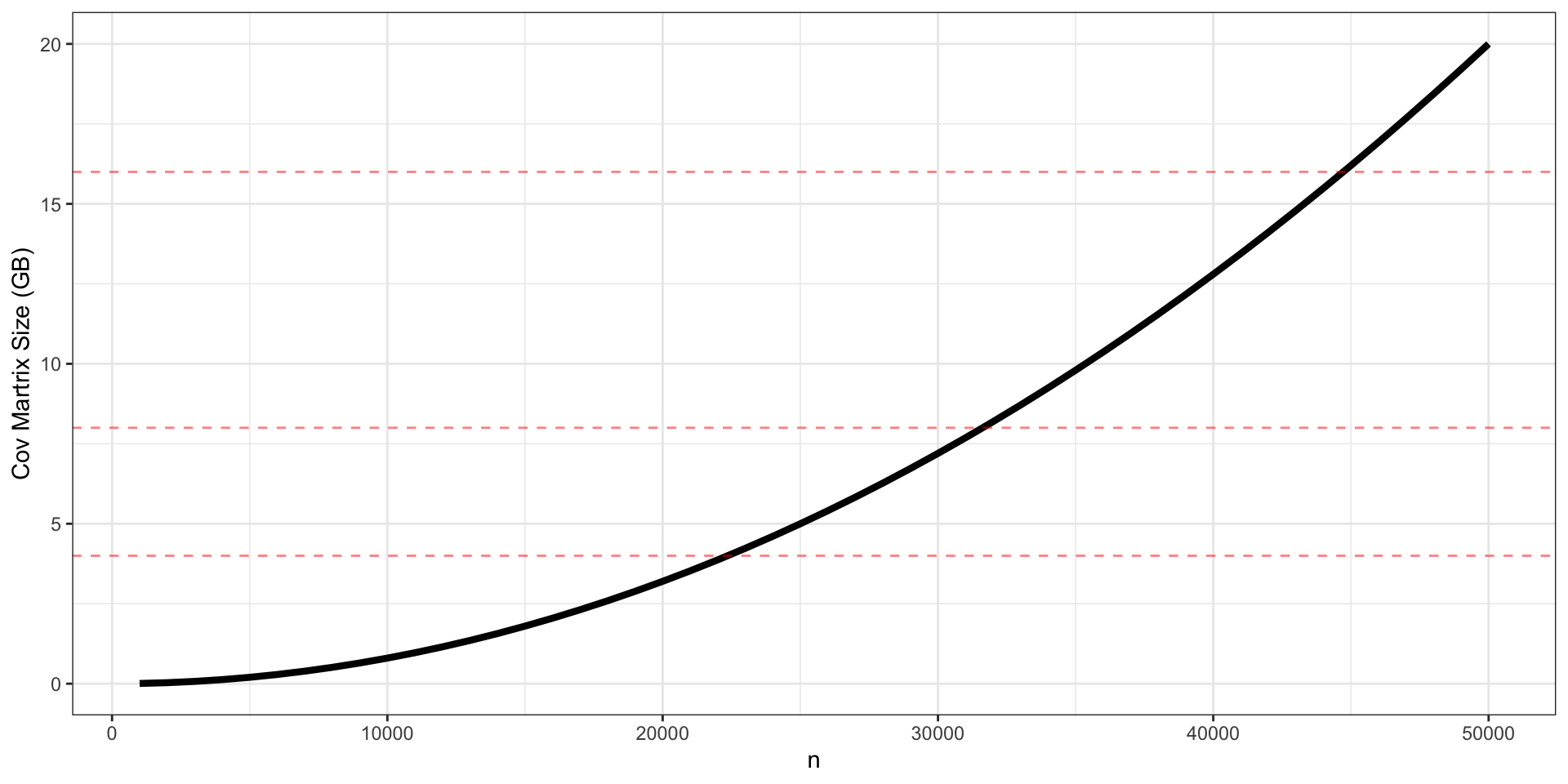
A general covariance is a dense \(n \times n\) matrix, meaning it will require \(n^2 \times\) 64-bits to store.
Other big hammers
bigGP is an R package written by Chris Paciorek (UC Berkeley), et al.
Specialized distributed implementation of linear algebra operation for GPs
Designed to run on large super computer clusters
Uses both shared and distributed memory
Able to fit models on the order of \(n = 65\)k (32 GB Cov. matrix)

More scalable solutions?
Spectral domain / basis functions
Covariance tapering
GMRF approximations
Low-rank approximations
Nearest-neighbor models
Low Rank Approximations
Low rank approximations in general
Lets look at the example of the singular value decomposition of a matrix,
\[ \underset{n \times m}{M} = \underset{n \times n}{U}\,\underset{n \times m}{\text{diag}(S)}\,\underset{m \times m}{V^{\,t}} \]
where \(U\) are the left singular vectors, \(V\) the right singular vectors, and \(S\) the singular values. Usually the singular values and vectors are ordered such that the singular values are in descending order.
The Eckart–Young theorem states that we can construct an approximatation of \(M\) with rank \(k\) by setting \(\tilde S\) to contain only the \(k\) largest singular values and all other values set to zero.
\[ \begin{aligned} \underset{n \times m}{\tilde M} &= \underset{n \times n}{U}\,\underset{n \times m}{\text{diag}(\tilde S)}\,\underset{m \times m}{V^{\,t}} \\ &= \underset{n \times k}{\tilde U}\,\underset{k \times k}{\text{diag}(\tilde S)}\,\underset{k \times m}{\tilde{V}^{\,t}} \end{aligned} \]
Example
\[ \begin{aligned} M &= \begin{pmatrix} 1.000 & 0.500 & 0.333 & 0.250 \\ 0.500 & 0.333 & 0.250 & 0.200 \\ 0.333 & 0.250 & 0.200 & 0.167 \\ 0.250 & 0.200 & 0.167 & 0.143 \\ \end{pmatrix} = U \, \text{diag}(S) \, V^{\,t} \\ U = V &= \begin{pmatrix} -0.79 & 0.58 & -0.18 & -0.03 \\ -0.45 & -0.37 & 0.74 & 0.33 \\ -0.32 & -0.51 & -0.10 & -0.79 \\ -0.25 & -0.51 & -0.64 & 0.51 \\ \end{pmatrix} \\ S &= \begin{pmatrix} 1.50 & 0.17 & 0.01 & 0.00 \end{pmatrix} \end{aligned} \]
Rank 2 approximation
\[ \begin{aligned} \tilde M &= \begin{pmatrix} -0.79 & 0.58 \\ -0.45 & -0.37 \\ -0.32 & -0.51 \\ -0.25 & -0.51 \\ \end{pmatrix} \begin{pmatrix} 1.50 & 0.00 \\ 0.00 & 0.17 \\ \end{pmatrix} \begin{pmatrix} -0.79 & -0.45 & -0.32 & -0.25 \\ 0.58 & -0.37 & -0.51 & -0.51 \\ \end{pmatrix} \\ &= \begin{pmatrix} 1.000 & 0.501 & 0.333 & 0.249 \\ 0.501 & 0.330 & 0.251 & 0.203 \\ 0.333 & 0.251 & 0.200 & 0.166 \\ 0.249 & 0.203 & 0.166 & 0.140 \\ \end{pmatrix} \end{aligned} \]
\[ \begin{aligned} M &= \begin{pmatrix} 1.000 & 0.500 & 0.333 & 0.250 \\ 0.500 & 0.333 & 0.250 & 0.200 \\ 0.333 & 0.250 & 0.200 & 0.167 \\ 0.250 & 0.200 & 0.167 & 0.143 \\ \end{pmatrix} \end{aligned} \]
Approximation Error
We can measure the error of the approximation using the Frobenius norm, \[ \lVert M-\tilde M\rVert_F = \left( \sum_{i=1}^m\sum_{j=1}^n (M_{ij}-\tilde M_{ij})^2\right)^{1/2} \]
\[ M-\tilde M = \begin{pmatrix} 0.00022 & -0.00090 & 0.00012 & 0.00077 \\ -0.00090 & 0.00372 & -0.00053 & -0.00317 \\ 0.00012 & -0.00053 & 0.00013 & 0.00039 \\ 0.00077 & -0.00317 & 0.00039 & 0.00277 \\ \end{pmatrix} \]
\[ \lVert M-\tilde M\rVert_F = 0.00674 \]
Strong dependence
For a covariance matrix with a large effective range,
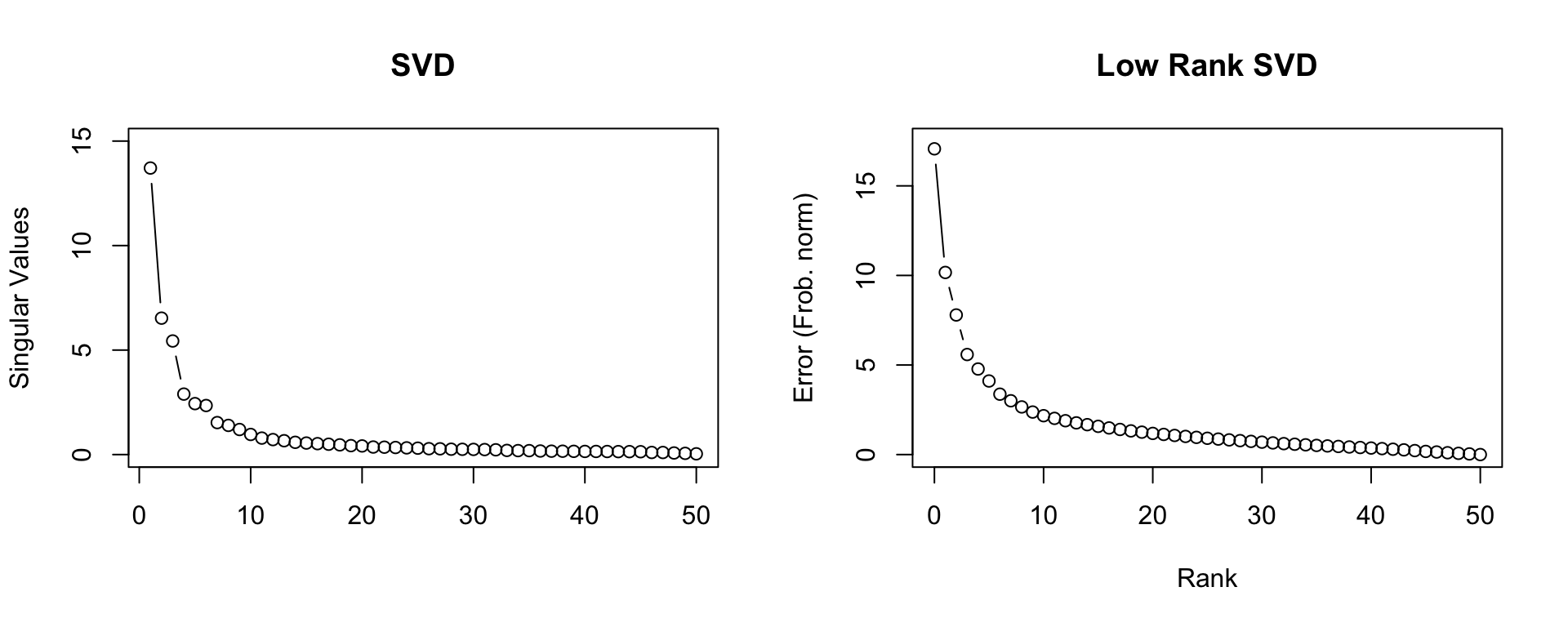
Weak dependence
For a covariance matrix with a large effective range,

How does this help?
There is an immensely useful linear algebra identity, the Sherman-Morrison-Woodbury formula, for the inverse (and determinant) of a decomposed matrix,
\[ \begin{aligned} \underset{n \times m}{M}^{-1} &= \left(\underset{n \times m}{A} + \underset{n \times k}{U} ~ \underset{k \times k}{S} ~ \underset{k \times m}{V^t}\right)^{-1} \\ &= A^{-1} - A^{-1} U \left(S^{-1}+V^{\,t} A^{-1} U\right)^{-1}V^{\,t} A^{-1}. \end{aligned} \]
How does this help?
Imagine that \(A = \text{diag}(A)\), then it is trivial to find \(A^{-1}\).
\(S^{-1}\) is \(k \times k\) which is hopefully small, or even better \(S = \text{diag}(S)\).
\(\left(S^{-1}+V^{\,t} A^{-1} U\right)\) is \(k \times k\) which is also small.
Aside - Determinant
Remember for any MVN distribution when evaluating the likelihood
\[ -\frac{1}{2} \log {|\Sigma|} - \frac{1}{2} (\boldsymbol{x}-\boldsymbol{\mu})' {\boldsymbol{\Sigma}^{-1}} (\boldsymbol{x}-\boldsymbol{\mu}) - \frac{n}{2}\log 2\pi \]
we need the inverse of \(\Sigma\) as well as its determinant.
For a full rank Cholesky decomposition we get the determinant for ``free’’. \[|M| = |LL^t| = \prod_{i=1}^n \left(\text{diag}(L)_i\right)^2\]
The Sherman-Morrison-Woodbury Determinant lemma gives us, \[ \begin{aligned} \det(M) &= \det({A} + {U} {S} {V^t}) \\ &= \det(S^{-1} + V^t A^{-1} U) ~ \det(S) ~ \det(A) \end{aligned} \]
Low rank approximations for GPs
For a standard spatial random effects model,
\[ y(\boldsymbol{s}) = x(\boldsymbol{s}) \, \boldsymbol{\beta} + w(\boldsymbol{s}) + \epsilon, \quad \epsilon \sim N(0,~\tau^2 I) \]
\[ w(\boldsymbol{s}) \sim \mathcal{N}(0,~\boldsymbol{\Sigma}(\boldsymbol{s})), \quad \boldsymbol{\Sigma}(\boldsymbol{s},\boldsymbol{s}')=\sigma^2\;\rho(\boldsymbol{s},\boldsymbol{s}'|\theta) \]
if we can replace \(\boldsymbol{\Sigma}(\boldsymbol{s})\) with a low rank approximation of the form \(\boldsymbol{\Sigma}(\boldsymbol{s}) \approx \boldsymbol{U}\,\boldsymbol{S}\,\boldsymbol{U}^t\) where
\(\boldsymbol{U}\) is \(n \times k\),
\(\boldsymbol{S}\) is \(k \times k\), and
\(A = \tau^2 I\) or a similar diagonal matrix
Predictive Processes
Gaussian Predictive Processes
For a rank \(k\) approximation,
- Pick \(k\) knot locations \(\boldsymbol{s}^\star\)
- Calculate knot covariance, \(\boldsymbol{\Sigma}(\boldsymbol{s}^\star)\), and knot cross-covariance, \(\boldsymbol{\Sigma}(\boldsymbol{s}, \boldsymbol{s}^\star)\)
- Approximate full covariance using
\[ \boldsymbol{\Sigma}(\boldsymbol{s}) \approx \underset{n \times k}{\boldsymbol{\Sigma}(\boldsymbol{s},\boldsymbol{s}^\star)} \, \underset{k \times k}{\boldsymbol{\Sigma}(\boldsymbol{s}^\star)^{-1}} \, \underset{k \times n}{\boldsymbol{\Sigma}(\boldsymbol{s}^\star,\boldsymbol{s})}. \]
- PPs systematically underestimates variance (\(\sigma^2\)) and inflate \(\tau^2\), Modified predictive processs corrects this using
\[ \begin{aligned} \boldsymbol{\Sigma}(\boldsymbol{s}) \approx & \boldsymbol{\Sigma}(\boldsymbol{s},\boldsymbol{s}^\star) \, \boldsymbol{\Sigma}(\boldsymbol{s}^\star)^{-1} \, \boldsymbol{\Sigma}(\boldsymbol{s}^\star,\boldsymbol{s}) \\ &+ \text{diag}\Big(\boldsymbol{\Sigma}(\boldsymbol{s}) - \boldsymbol{\Sigma}(\boldsymbol{s},\boldsymbol{s}^\star) \, \boldsymbol{\Sigma}(\boldsymbol{s}^\star)^{-1} \, \boldsymbol{\Sigma}(\boldsymbol{s}^\star,\boldsymbol{s})\Big). \end{aligned} \]
Example
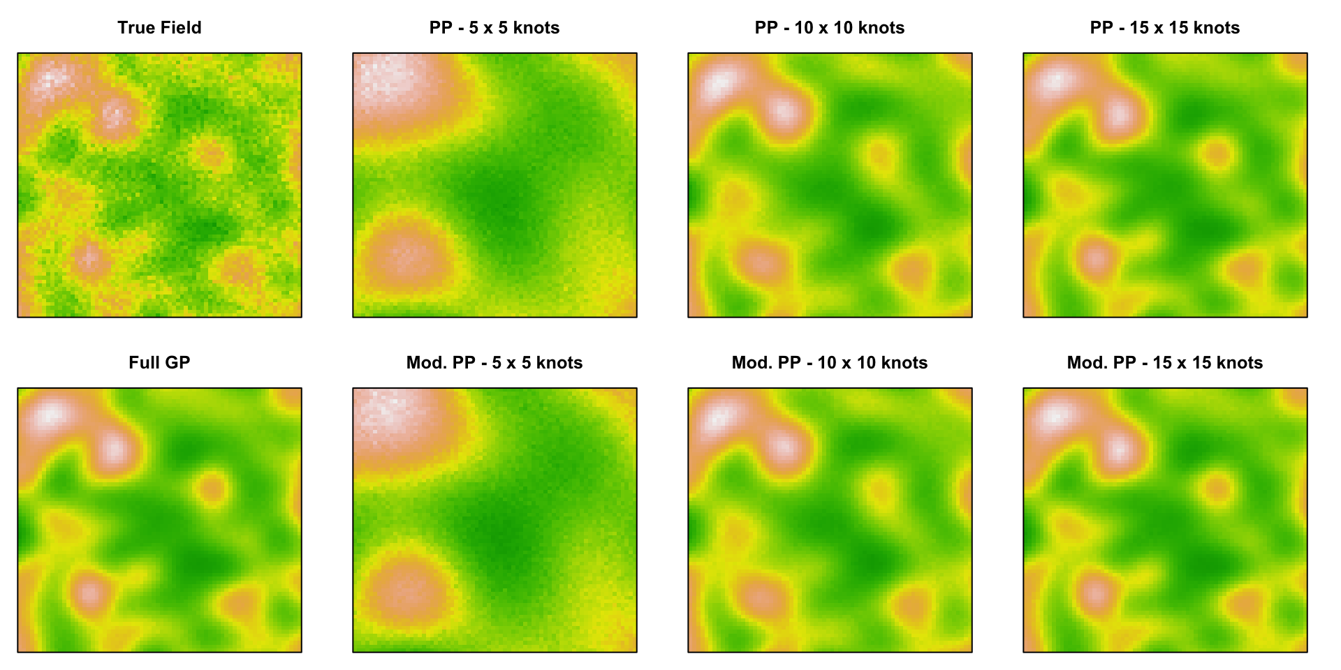
Below we have a surface generate from a squared exponential Gaussian Process where \[ \{\Sigma\}_{ij} = \sigma^2 \exp\left(-(\phi\,d)^2\right) + \tau^2 I \] \[ \sigma^2 = 1 \quad \phi=9 \quad \tau^2 = 0.1 \]

Predictive Process Model Results
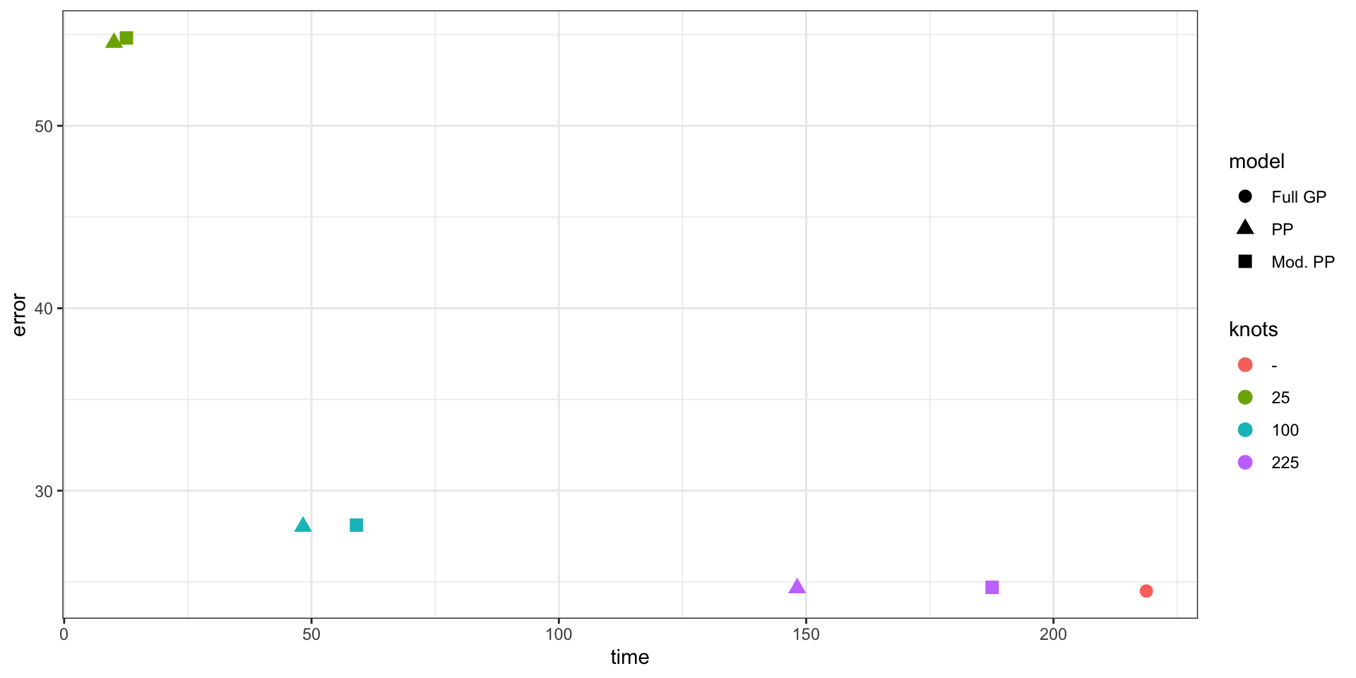
Performance
Parameter Estimates

Random Projections
Low Rank via Random Projections
- Starting with an matrix \(\underset{m \times n}{\boldsymbol{A}}\).
- Draw a Gaussian random matrix \(\underset{n \times k+p}{\boldsymbol{\Omega}}\).
- Form \(\boldsymbol{Y} = \boldsymbol{A}\,\boldsymbol{\Omega}\) and compute its QR factorization \(\boldsymbol{Y} = \boldsymbol{Q}\,\boldsymbol{R}\)
- Form \(\boldsymbol{B}=\boldsymbol{Q}'\,\boldsymbol{A}\).
- Compute the SVD of \(\boldsymbol{B} = \boldsymbol{\hat{U}}\,\boldsymbol{S}\,\boldsymbol{V}'\).
- Form the matrix \(\boldsymbol{U} = \boldsymbol{Q} \, \boldsymbol{\hat{U}}\).
- Form \(\boldsymbol{\tilde{A}} = \boldsymbol{U}\boldsymbol{S}\boldsymbol{V}'\)
Resulting approximation has a bounded expected error,
\[ E| \boldsymbol{A} - \boldsymbol{U}\boldsymbol{S}\boldsymbol{V}'\|_F \leq \left[1 + \frac{4\sqrt{k+p}}{p-1} \sqrt{\min(m,n)} \right] \sigma_{k+1}. \]
Random Matrix Low Rank Approxs and GPs
The preceding algorithm can be modified slightly to take advantage of the positive definite structure of a covariance matrix.
Starting with an \(n \times n\) covariance matrix \(\boldsymbol{A}\).
Draw Gaussian random matrix \(\underset{n \times k+p}{\boldsymbol{\Omega}}\).
Form \(\boldsymbol{Y} = \boldsymbol{A}\,\boldsymbol{\Omega}\) and compute its QR factorization \(\boldsymbol{Y} = \boldsymbol{Q}\,\boldsymbol{R}\)
Form the \(\boldsymbol{B}=\boldsymbol{Q}'\,\boldsymbol{A} \, \boldsymbol{Q}\).
Compute the eigen decomposition of \(\boldsymbol{B} = \boldsymbol{\hat{U}}\,\boldsymbol{S}\,\boldsymbol{\hat{U}}'\).
Form the matrix \(\boldsymbol{U} = \boldsymbol{Q} \, \boldsymbol{\hat{U}}\).
Once again we have a bound on the error,
\[ E \|\boldsymbol{A} - \boldsymbol{U}\boldsymbol{S}\boldsymbol{U}'\|_F \lesssim c \cdot \sigma_{k+1}. \]
Low Rank Approximations and GPUs
Both predictive process and random matrix low rank approximations are good candidates for acceleration using GPUs.
Both use Sherman-Woodbury-Morrison to calculate the inverse (involves matrix multiplication, addition, and a small matrix inverse).
Predictive processes involves several covariance matrix calculations (knots and cross-covariance) and a small matrix inverse.
Random matrix low rank approximations involves a large matrix multiplication (\(\boldsymbol{A}\,\boldsymbol{\Omega}\)) and several small matrix decompositions (QR, eigen).
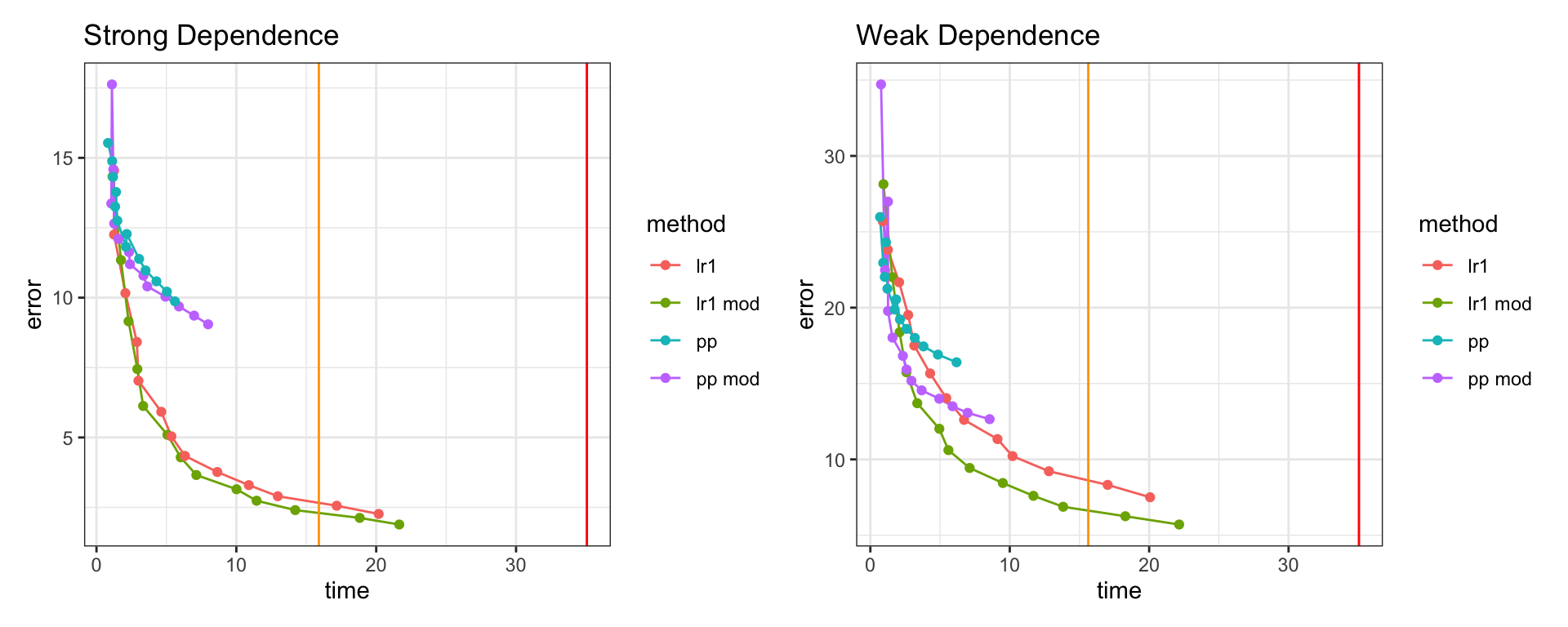
Comparison \(n=15,000,\;k=\{100,\ldots,4900\}\)
Rand. Projection LR Depositions for Prediction
This approach can also be used for prediction, if we want to sample
\[ \boldsymbol{y} \sim \mathcal{N}(0,\boldsymbol{\Sigma}) \] \[ \Sigma \approx \boldsymbol{U} \boldsymbol{S} \boldsymbol{U}^t = (\boldsymbol{U} \boldsymbol{S}^{1/2} \boldsymbol{U}^t)(\boldsymbol{U} \boldsymbol{S}^{1/2} \boldsymbol{U}^t)^t \]
then
\[ y_{\text{pred}} = (\boldsymbol{U}\, \boldsymbol{S}^{1/2}\,\boldsymbol{U}^t) \times \boldsymbol{Z} \text{ where } Z_i \sim \mathcal{N}(0,1) \]
because \(\boldsymbol{U}^t \, \boldsymbol{U} = I\) since \(\boldsymbol{U}\) is an orthogonal matrix.

\[ n=1000, \quad p=10000 \]
Sta 344 - Fall 2022