Spatial GLM + Point Reference Spatial Data
Lecture 21
Spatial GLM Models
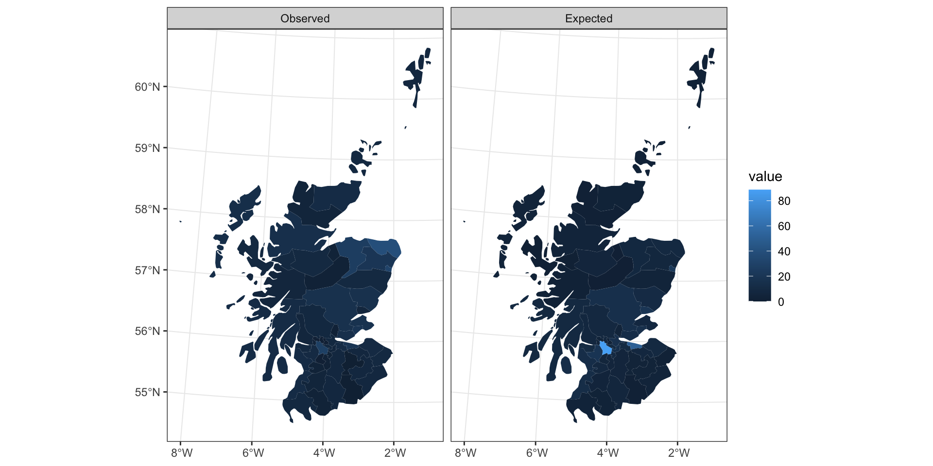
Scottish Lip Cancer Data
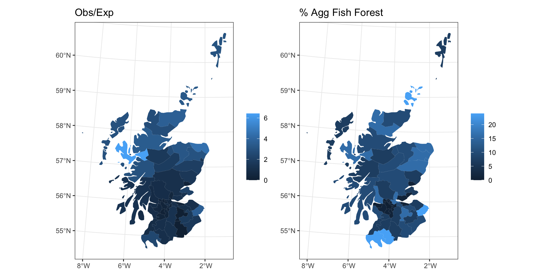
Neighborhood / weight matrix
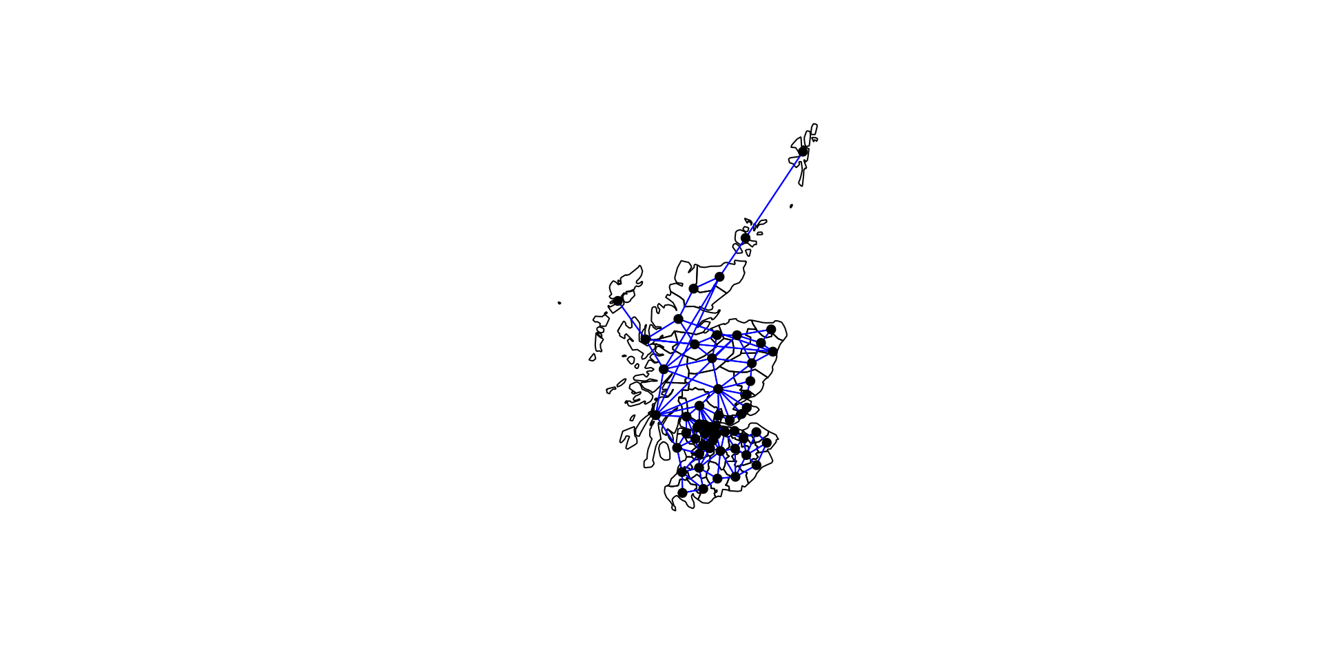
Moran’s I
    Moran I test under randomisation

data:  lip_cancer$Observed
weights: listw

Moran I statistic standard deviate = 4.5416,
p-value = 2.792e-06
alternative hypothesis: greater
sample estimates:
Moran I statistic       Expectation
      0.311975396      -0.018181818
         Variance
      0.005284831
    Moran I test under randomisation

data:  lip_cancer$Observed/lip_cancer$Expected
weights: listw

Moran I statistic standard deviate = 8.2916,
p-value < 2.2e-16
alternative hypothesis: greater
sample estimates:
Moran I statistic       Expectation
      0.589795225      -0.018181818
         Variance
      0.005376506
GLM
Call:
glm(formula = Observed ~ offset(log(Expected)) + pcaff, family = "poisson",
    data = lip_cancer)

Deviance Residuals:
    Min       1Q   Median       3Q      Max
-4.7632  -1.2156   0.0967   1.3362   4.7130

Coefficients:
             Estimate Std. Error z value Pr(>|z|)
(Intercept) -0.542268   0.069525   -7.80 6.21e-15
pcaff        0.073732   0.005956   12.38  < 2e-16

(Intercept) ***
pcaff       ***
---
Signif. codes:
0 '***' 0.001 '**' 0.01 '*' 0.05 '.' 0.1 ' ' 1

(Dispersion parameter for poisson family taken to be 1)

    Null deviance: 380.73  on 55  degrees of freedom
Residual deviance: 238.62  on 54  degrees of freedom
AIC: 450.6

Number of Fisher Scoring iterations: 5
GLM Fit
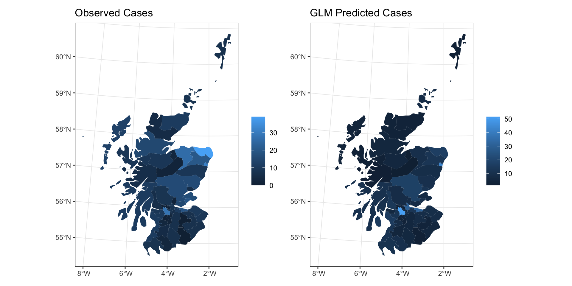
GLM Fit
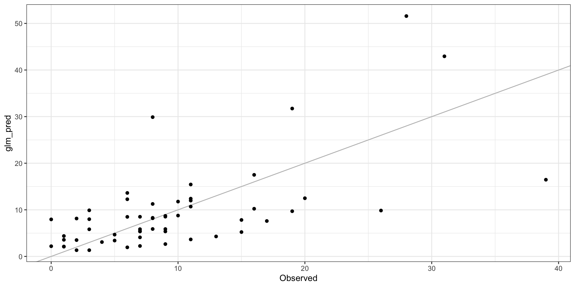
GLM Residuals
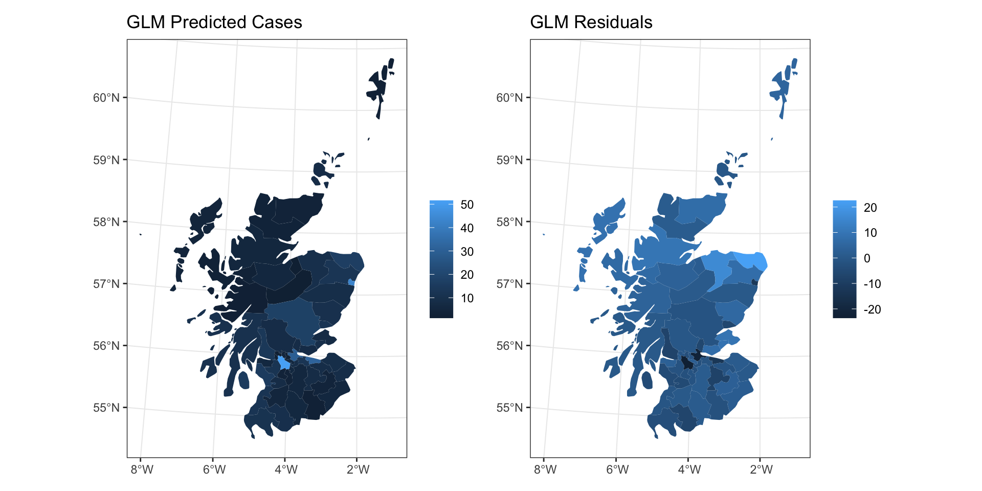
Model Results
    Moran I test under randomisation

data:  lip_cancer$glm_resid
weights: listw

Moran I statistic standard deviate = 4.8186,
p-value = 7.228e-07
alternative hypothesis: greater
sample estimates:
Moran I statistic       Expectation
      0.333403223      -0.018181818
         Variance
      0.005323717
A hierachical model for lip cancer
We have observed counts of lip cancer for 56 districts in Scotland. Let \(y_i\) represent the number of lip cancer for district \(i\).
\[\begin{aligned} y_i &\sim \text{Poisson}(\lambda_i) \\ \\ \log(\lambda_i) &= \log(E_i) + x_i \beta + \omega_i \\ \\ \boldsymbol{\omega} &\sim \mathcal{N}(\boldsymbol{0},~\sigma^2(\boldsymbol{D}-\phi\,\boldsymbol{A})^{-1}) \end{aligned}\]
where \(E_i\) is the expected counts for each region (and serves as an offset).
Data prep & CAR model
car_model = "
data {
  int<lower=0> N;
  int<lower=0> p;
  int<lower=0> y[N];
  matrix[N,N] A;
  matrix[N,p] X;
  vector[N] offset;
}
transformed data {
  vector[N] nb = A * rep_vector(1, N);
  matrix[N,N] D = diag_matrix(nb);
}
parameters {
  vector[N] w_s;
  vector[p] beta;
  real<lower=0> sigma2;
  real<lower=0,upper=1> phi;
}
transformed parameters {
  vector[N] eta = log(offset) + X * beta + w_s;
}
model {
  matrix[N,N] Sigma_inv = (D - phi * A) / sigma2;
  w_s ~ multi_normal_prec(rep_vector(0,N), Sigma_inv);

  beta ~ normal(0,10);
  sigma2 ~ cauchy(0,5);

  y ~ poisson_log(eta);
}
"
CAR Fitting
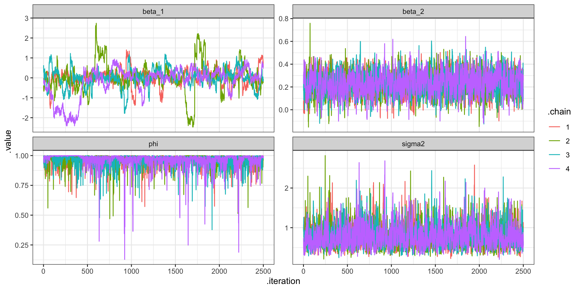
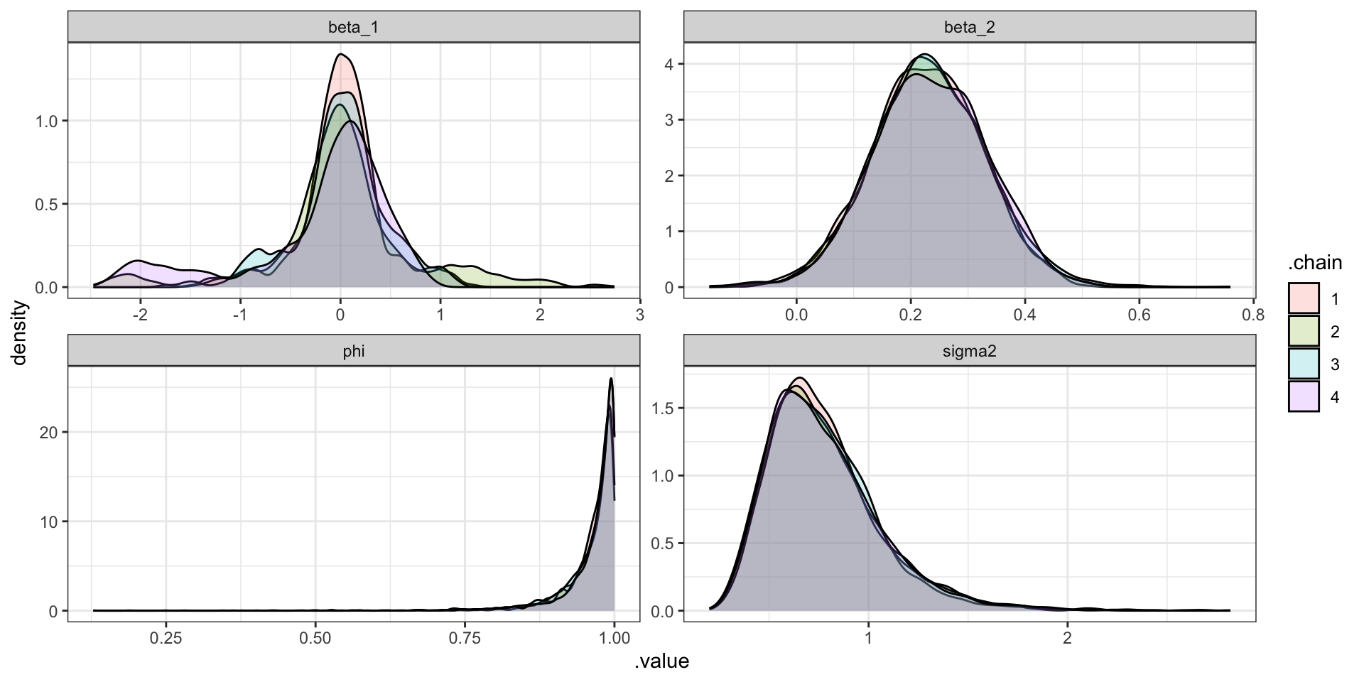
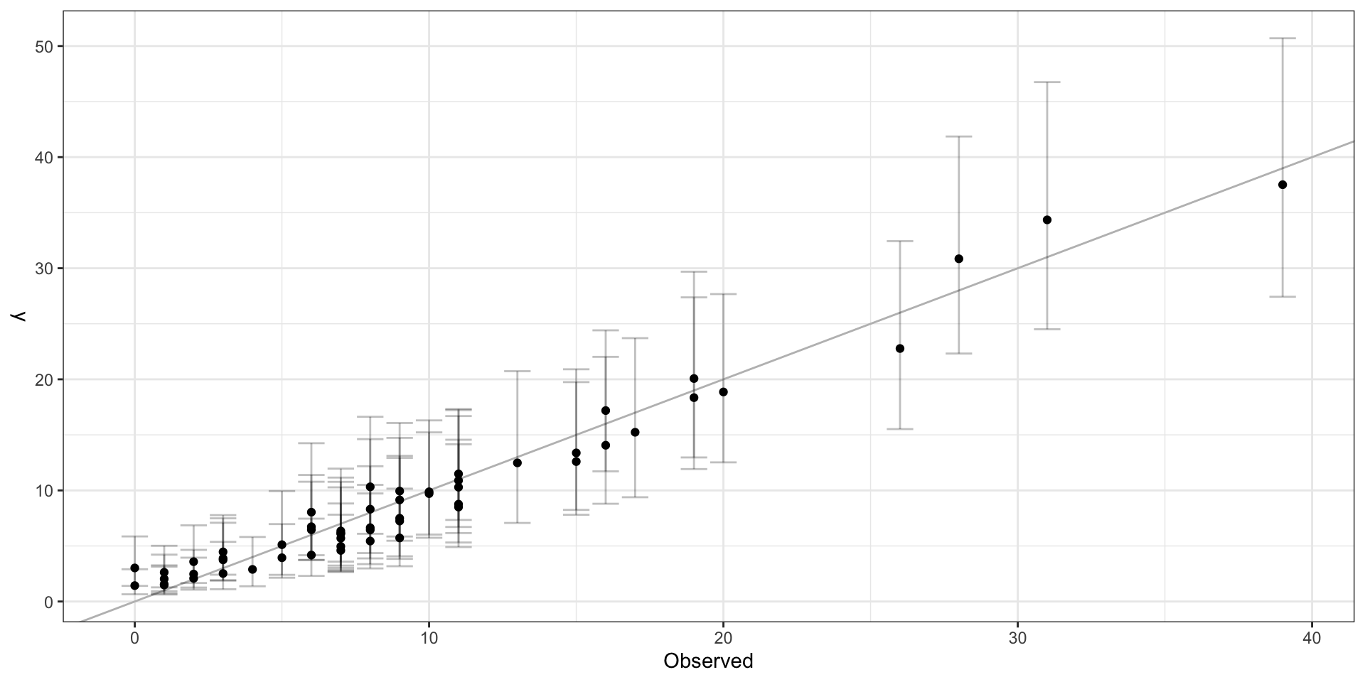
CAR Predictions (\(\hat\lambda\))
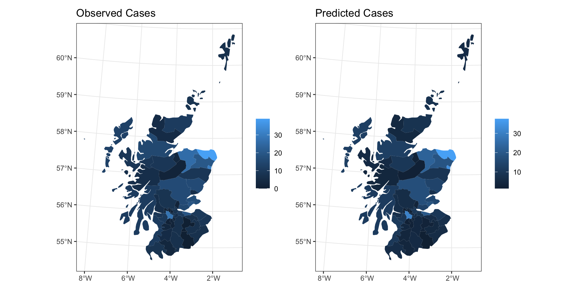
CAR Predictions
CAR Residuals
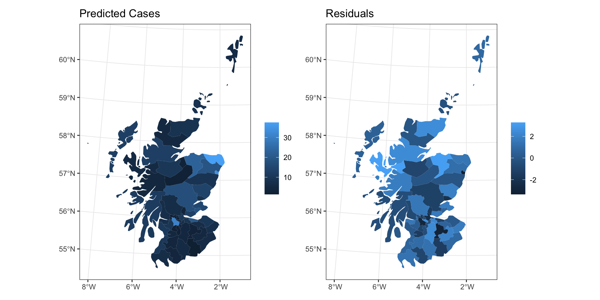
CAR Results
    Moran I test under randomisation

data:  car_lip_cancer$Observed - car_lip_cancer$y_pred
weights: listw

Moran I statistic standard deviate =
0.73353, p-value = 0.2316
alternative hypothesis: greater
sample estimates:
Moran I statistic       Expectation
      0.036963635      -0.018181818
         Variance
      0.005651802
Latent spatial process
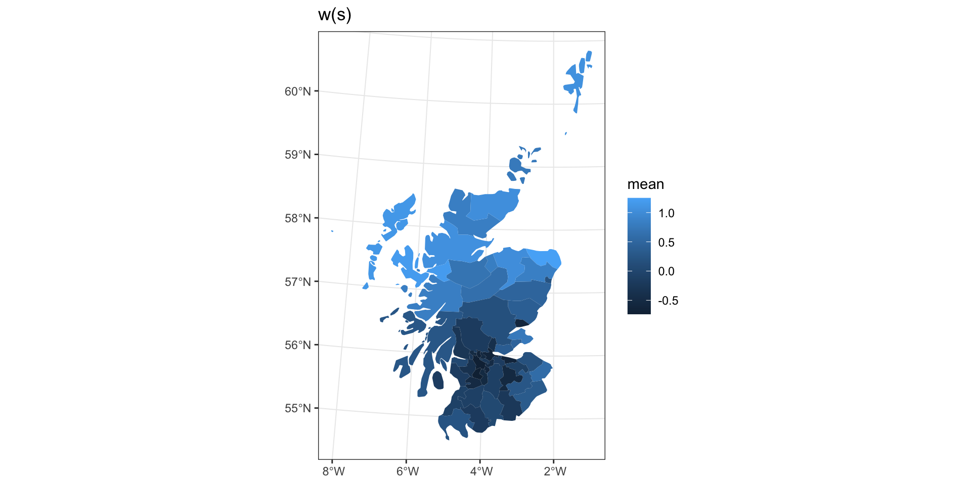
Intrinsic Autoregressive Model (IAR)
Predictions
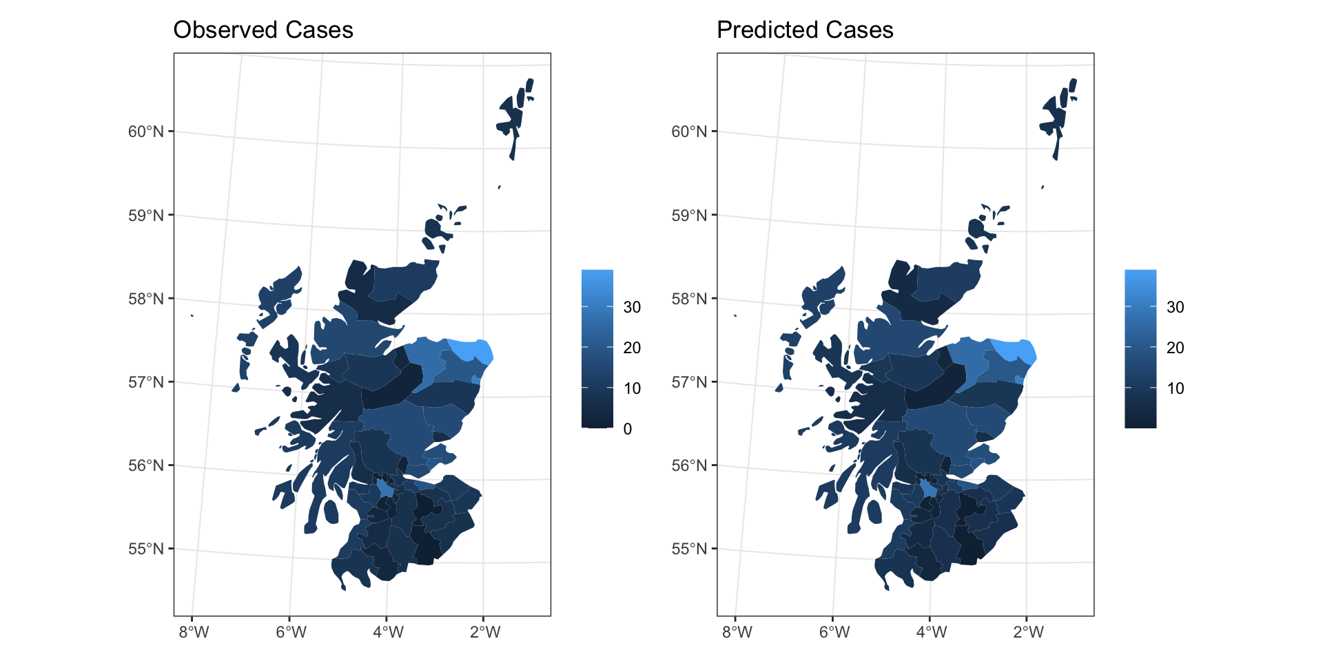
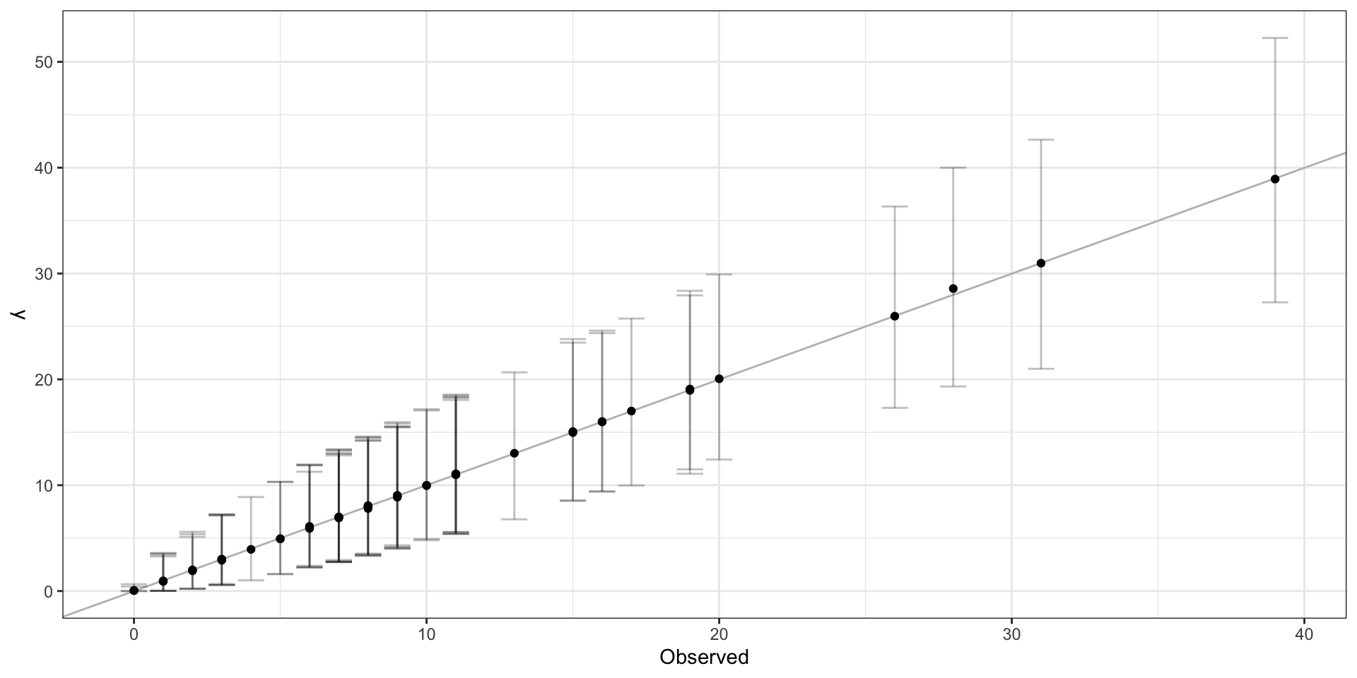
Observed vs predicted
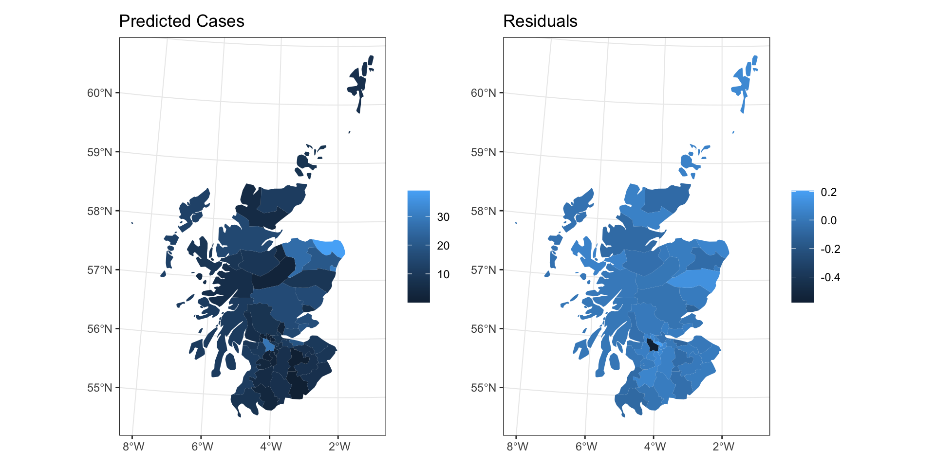
Residuals
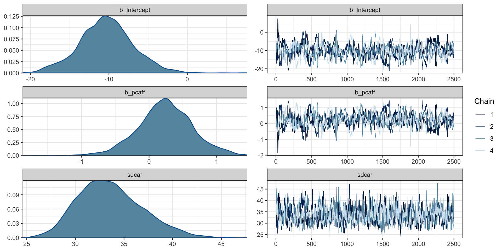
IAR Results
[1] 0.09762396
    Moran I test under randomisation

data:  iar_pred$resid
weights: listw

Moran I statistic standard deviate = 2.5724,
p-value = 0.005051
alternative hypothesis: greater
sample estimates:
Moran I statistic       Expectation
      0.131306700      -0.018181818
         Variance
      0.003377189
Point Referenced Data
Example - PM2.5 from CSN
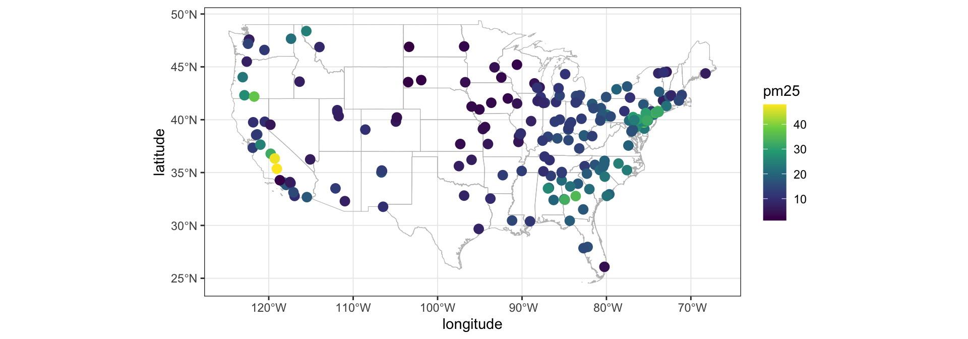
The Chemical Speciation Network are a series of air quality monitors run by EPA (221 locations in 2007). We’ll look at a subset of the data from Nov 11th, 2007 (n=191) for just PM2.5.
# A tibble: 191 × 5
       site longitude latitude date
      <int>     <dbl>    <dbl> <dttm>
 1 10730023     -86.8     33.6 2007-11-14 00:00:00
 2 10732003     -86.9     33.5 2007-11-14 00:00:00
 3 10890014     -86.6     34.7 2007-11-14 00:00:00
 4 11011002     -86.3     32.4 2007-11-14 00:00:00
 5 11130001     -85.0     32.5 2007-11-14 00:00:00
 6 40139997    -112.      33.5 2007-11-14 00:00:00
 7 40191028    -111.      32.3 2007-11-14 00:00:00
 8 51190007     -92.3     34.8 2007-11-14 00:00:00
 9 60070002    -122.      39.8 2007-11-14 00:00:00
10 60190008    -120.      36.8 2007-11-14 00:00:00
# … with 181 more rows, and 1 more variable:
#   pm25 <dbl>
Aside - Splines


Splines in 1d - Smoothing Splines
These are a mathematical analogue to the drafting splines represented using a penalized regression model.
We want to find a function \(f(x)\) that best fits our observed data \(\boldsymbol{y} = y_1, \ldots, y_n\) while being smooth.
\[ \underset{f(x)}{\arg\min} ~ \sum_{i=1}^n\left(y_i - f(x_i)\right)^2 + \lambda \int_{-\infty}^\infty f''(x)^2 ~ dx \]
Interestingly, this minimization problem has an exact solution which is given by a mixture of weighted natural cubic splines (cubic splines that are linear in the tails) with knots at the observed data locations (\(x\)s).
Splines in 2d - Thin Plate Splines
Now imagine we have observed data of the form \((x_i, y_i, z_i)\) where we wish to predict \(z_i\) given \(x_i\) and \(y_i\) for all \(i\). We can extend the smoothing spline model in two dimensions,
\[ \underset{f(x,y)}{\arg\min} ~~ \sum_{i=1}^n (z_i-f(x_i,y_i))^2 + \lambda \int_{-\infty}^\infty \int_{-\infty}^\infty \left(\frac{\partial^2 f}{\partial x^2} + 2 \frac{\partial^2 f}{\partial x \, \partial y} + \frac{\partial^2 f}{\partial y^2} \right) dx\, dy\]
The solution to this equation has a natural representation using a weighted sum of radial basis functions with knots at the observed data locations (\(\boldsymbol{x_i}\))
\[ f(\boldsymbol{x}) = \sum_{i=1}^n w_i ~ d(\boldsymbol{x}, \boldsymbol{x_i})^2 \log d(\boldsymbol{x}, \boldsymbol{x_i}).\]
Prediction locations
Fitting a TPS
coords = select(csn, long=longitude, lat=latitude) |>
  as.matrix()
(tps = fields::Tps(x = coords, Y=csn$pm25, lon.lat=TRUE))
Call:
fields::Tps(x = coords, Y = csn$pm25, lon.lat = TRUE)
Number of Observations: 191
Number of parameters in the null space 3
Parameters for fixed spatial drift 3
Model degrees of freedom: 64
Residual degrees of freedom: 127
GCV estimate for tau: 4.461
MLE for tau: 4.286
MLE for sigma: 15.35
lambda 1.2
User supplied sigma NA
User supplied tau^2 NA
Summary of estimates:
lambda trA GCV tauHat
GCV 1.196496 63.97784 29.91791 4.460553
GCV.model NA NA NA NA
GCV.one 1.196496 63.97784 29.91791 4.460553
RMSE NA NA NA NA
pure error NA NA NA NA
REML 2.411838 50.52688 30.58992 4.743174
-lnLike Prof converge
GCV 612.4247 5
GCV.model NA NA
GCV.one NA 5
RMSE NA NA
pure error NA NA
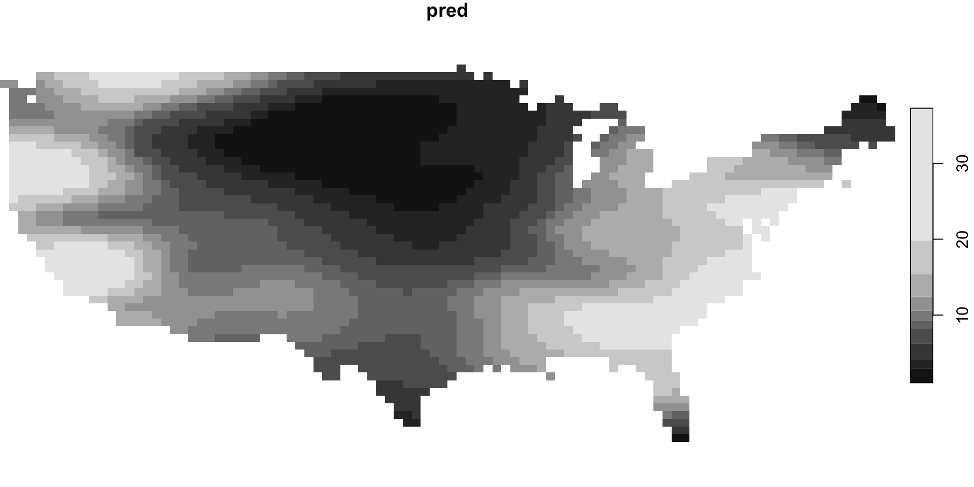
REML 611.0553 6Predictions
Gaussin Process Models / Kriging
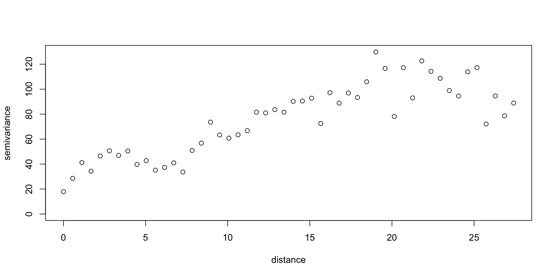
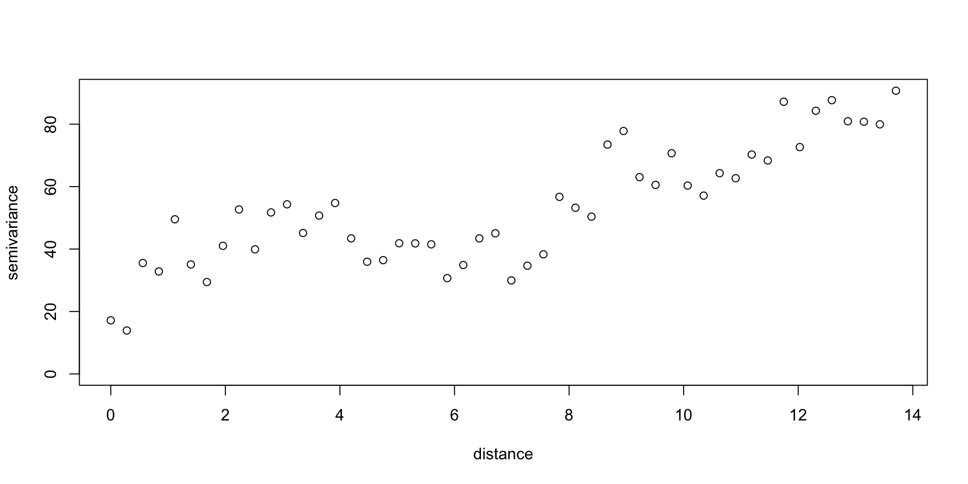
Variogram
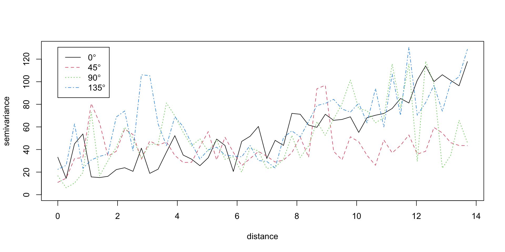
Isotropy / Anisotropy
GP Spatial Model
If we assume that our data is stationary and isotropic then we can use a Gaussian Process model to fit the data. We will assume an exponential covariance structure.
\[ \boldsymbol{y} \sim \mathcal{N}(\boldsymbol{\mu},~\Sigma) \] \[ \{\Sigma\}_{ij} = \sigma^2 \exp(- l \, \lVert s_i - s_j\lVert) + \sigma^2_n \, 1_{i=j} \]
we can also view this as a spatial random effects model where
\[ y(\boldsymbol{s}) = \mu(\boldsymbol{s}) + w(\boldsymbol{s}) + \epsilon(\boldsymbol{s}) \\ w(\boldsymbol{s}) \sim \mathcal{N}(0,\Sigma') \\ \epsilon(s_i) \sim \mathcal{N}(0,\sigma^2_n) \\ \{\Sigma'\}_{ij} = \sigma^2 \exp(- r \, \lVert s_i - s_j\lVert) \]
Fitting with gplm() (spBayes)
max_range = max(dist(csn[,c("longitude", "latitude")])) / 4

m = gplm(
  pm25~1, data = csn, coords=c("longitude", "latitude"),
  cov_model = "exponential",
  starting = list(phi = 3/3, sigma.sq = 33, tau.sq = 17),
  tuning = list("phi"=0.1, "sigma.sq"=0.1, "tau.sq"=0.1),
  priors = list(
    phi.Unif = c(3/max_range, 3/(0.5)),
    sigma.sq.IG = c(2, 2),
    tau.sq.IG = c(2, 2)
  ),
  thin=10,
  verbose=TRUE
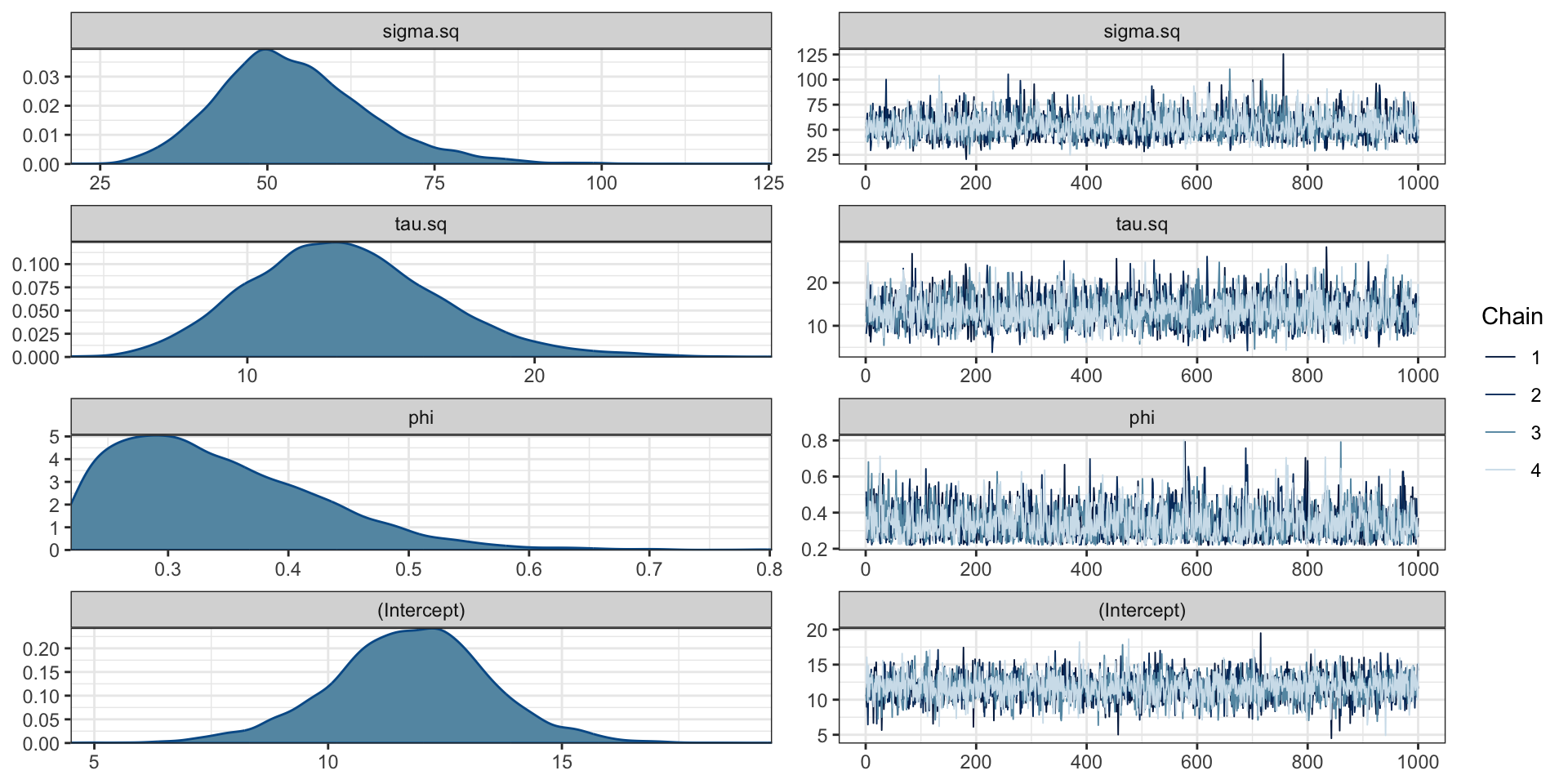
)# A gplm model (spBayes spLM) with 4 chains, 4 variables, and 4000 iterations.
# A tibble: 4 × 10
variable mean median sd mad q5
<chr> <dbl> <dbl> <dbl> <dbl> <dbl>
1 sigma.sq 54.0 52.9 11.3 10.4 37.7
2 tau.sq 13.4 13.2 3.33 3.20 8.28
3 phi 0.341 0.325 0.0848 0.0835 0.232
4 (Intercept) 11.8 11.8 1.71 1.59 8.87
# … with 4 more variables: q95 <dbl>, rhat <dbl>,
# ess_bulk <dbl>, ess_tail <dbl>Parameter values
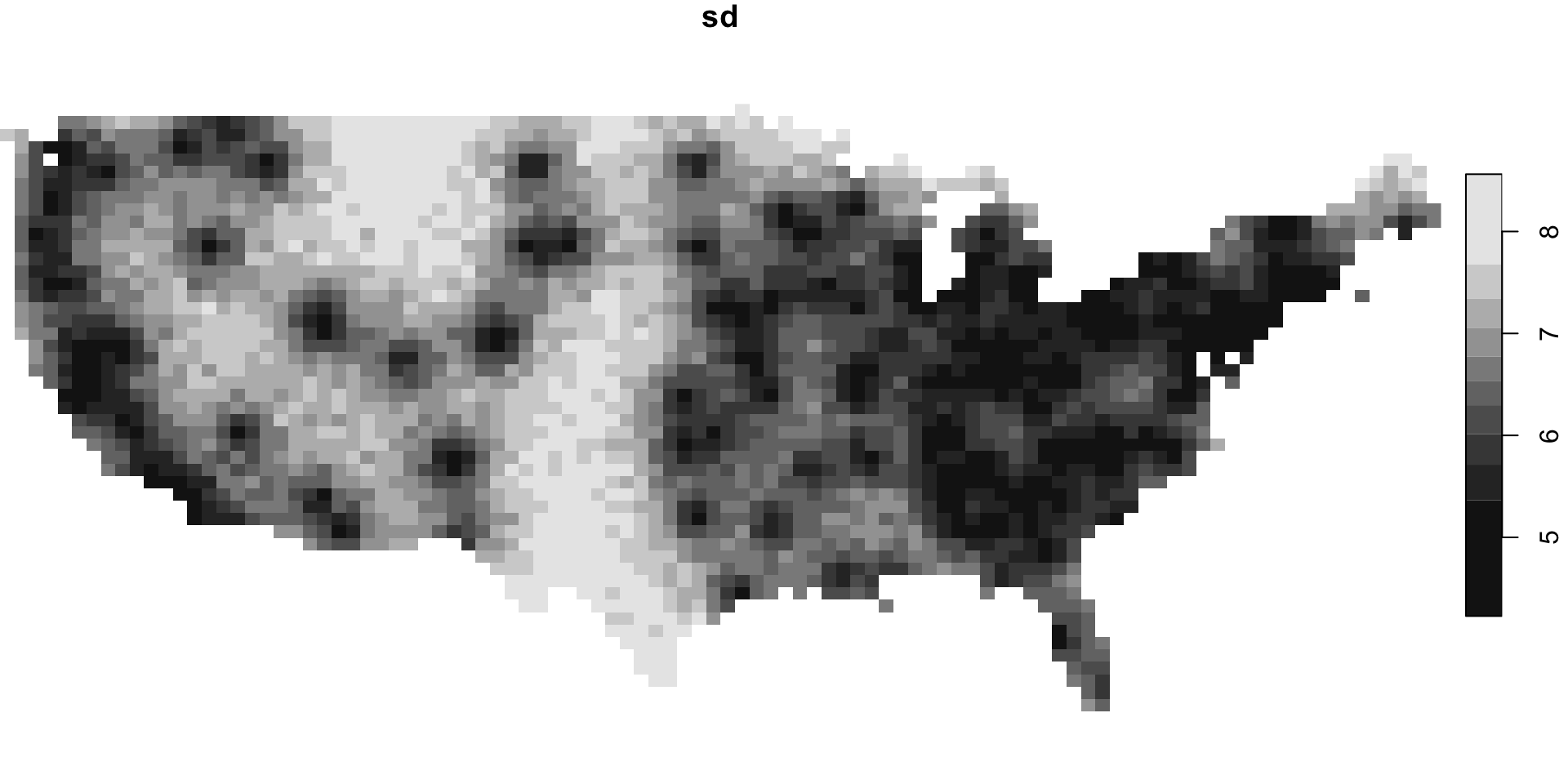
Predictions
# A draws_matrix: 1000 iterations, 4 chains, and 2828 variables
    variable
draw  y[1]   y[2] y[3] y[4] y[5]  y[6] y[7] y[8]
  1  14.03 -4.073 15.0  4.8 -8.8  7.84   21  4.9
  2  11.71  0.052 10.2  5.8 11.3 14.58   20 10.7
  3  -3.37 17.307 18.4 20.2 23.7 28.46    9 20.4
  4   7.31  2.500  4.6  7.3 23.7 14.63   15 11.8
  5   0.47 10.014 10.4 17.2 14.6 11.17   10 10.0
  6   7.57 11.004 10.6  9.2 10.6 14.56   23 10.0
  7   7.16  6.791 12.8  5.0 22.4  0.88   16 20.1
  8  16.54  9.611  1.8 23.9 23.9 19.23   38 10.0
  9  16.03  3.135 23.7  1.1 12.4 13.10   34 20.1
  10 14.14  0.638 13.7  8.7 -4.9 11.37   18 13.5
# ... with 3990 more draws, and 2820 more variables
Sta 344 - Fall 2022
