Fitting CAR and SAR Models

Lecture 20

Dr. Colin Rundel

Fitting areal models

Revised SAR Model

• Formula Model

\[ y(s_i) = X_{i\cdot}\beta + \phi \sum_{j=1}^n D^{-1}_{jj} \, A_{ij} \, \big(y(s_j) - X_{j\cdot}\beta\big) + \epsilon_i \] \[ \boldsymbol{\epsilon} \sim N(\boldsymbol{0},\, \sigma^2 \boldsymbol{D}^{-1}) \]

• Joint Model

\[ \boldsymbol{y} \sim N\left(\boldsymbol{X}\boldsymbol{\beta}, (\boldsymbol{I} - \phi \boldsymbol{D}^{-1} \boldsymbol{A})^{-1} \sigma^2 \boldsymbol{D}^{-1} \big((\boldsymbol{I} - \phi \boldsymbol{D}^{-1} \boldsymbol{A})^{-1}\big)^t \right) \]

Revised CAR Model

• Conditional Model

\[ y(s_i)|\boldsymbol{y}_{-s_i} \sim N\left(X_{i\cdot}\beta + \phi\sum_{j=1}^n \frac{A_{ij}}{D_{ii}} ~ \big(y(s_j)-X_{j\cdot}\beta\big),~ \sigma^2 D^{-1}_{ii} \right) \]

• Joint Model

\[\boldsymbol{y} \sim N(\boldsymbol{X}\boldsymbol{\beta},~\sigma^2(\boldsymbol{D}-\phi \boldsymbol{A})^{-1})\]

Example - NC SIDS

ggplot() + geom_sf(data=nc, aes(fill=SID74/BIR74*1000))

Using spdep + spatialreg

library(spdep)

A = st_touches(nc, sparse=FALSE)
(listW = spdep::mat2listw(A))

Characteristics of weights list object:
Neighbour list object:
Number of regions: 100 
Number of nonzero links: 490 
Percentage nonzero weights: 4.9 
Average number of links: 4.9 

Weights style: M 
Weights constants summary:
    n    nn  S0  S1    S2
M 100 10000 490 980 10696

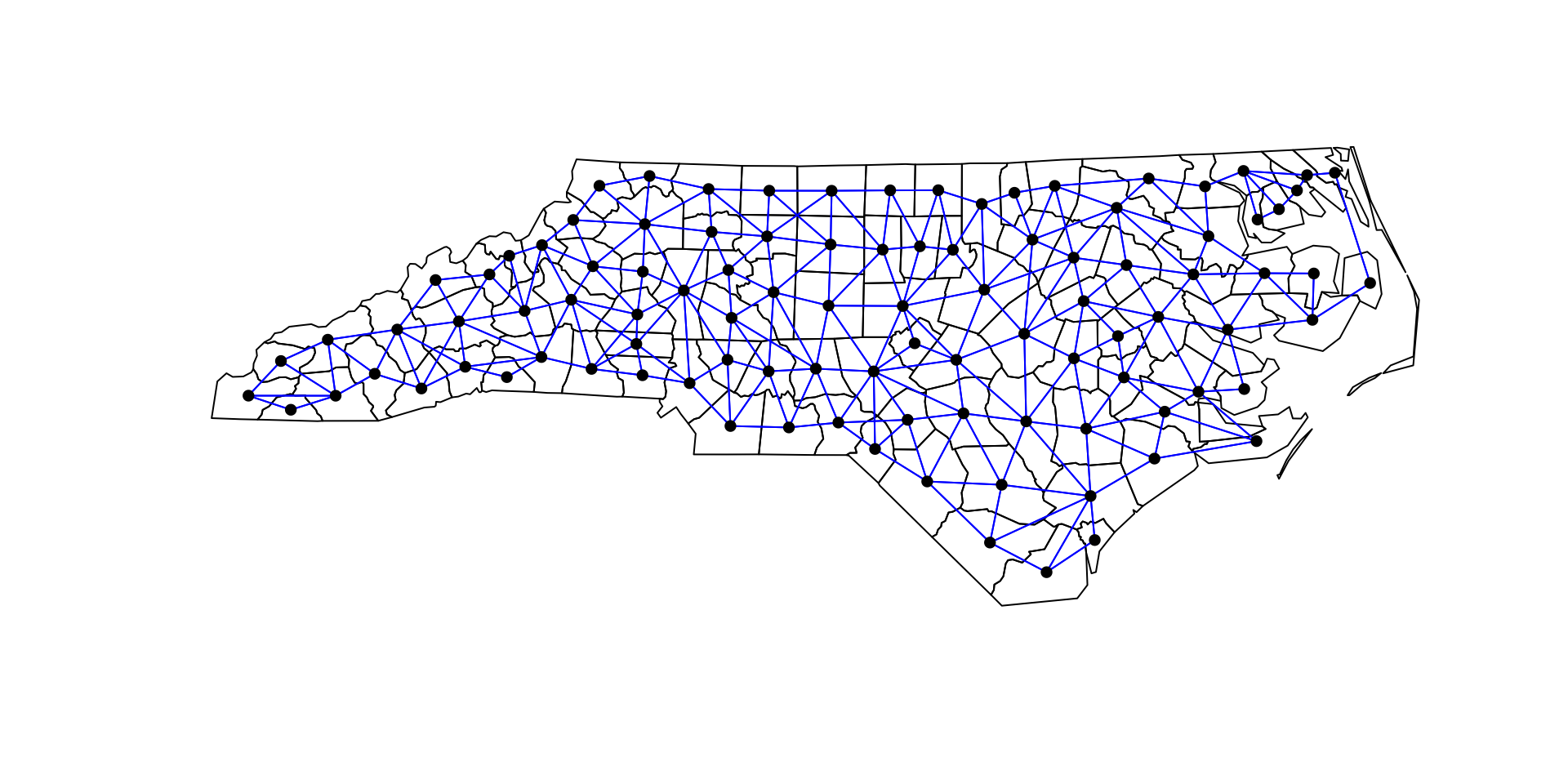
Plotting listw

nc_coords = nc %>% st_centroid() %>% st_coordinates()

plot(st_geometry(nc))
plot(listW, nc_coords, add=TRUE, col="blue", pch=16)

Moran’s I

spdep::moran.test(nc$SID74, listW)

    Moran I test under randomisation

data:  nc$SID74  
weights: listW    

Moran I statistic standard deviate = 2.1707,
p-value = 0.01498
alternative hypothesis: greater
sample estimates:
Moran I statistic       Expectation 
      0.119089049      -0.010101010 
         Variance 
      0.003542176 

spdep::moran.test(1000*nc$SID74/nc$BIR74, listW)

    Moran I test under randomisation

data:  1000 * nc$SID74/nc$BIR74  
weights: listW    

Moran I statistic standard deviate = 3.6355,
p-value = 0.0001387
alternative hypothesis: greater
sample estimates:
Moran I statistic       Expectation 
      0.210046454      -0.010101010 
         Variance 
      0.003666802 

Geary’s C

spdep::geary.test(nc$SID74, listW)

    Geary C test under randomisation

data:  nc$SID74 
weights: listW 

Geary C statistic standard deviate =
0.91949, p-value = 0.1789
alternative hypothesis: Expectation greater than statistic
sample estimates:
Geary C statistic       Expectation 
       0.88988684        1.00000000 
         Variance 
       0.01434105 

spdep::geary.test(1000*nc$SID74/nc$BIR74, listW)

    Geary C test under randomisation

data:  1000 * nc$SID74/nc$BIR74 
weights: listW 

Geary C statistic standard deviate = 3.0989,
p-value = 0.0009711
alternative hypothesis: Expectation greater than statistic
sample estimates:
Geary C statistic       Expectation 
       0.67796679        1.00000000 
         Variance 
       0.01079878 

CAR Model

nc_car = spatialreg::spautolm(
  formula = 1000*SID74/BIR74 ~ 1, data = nc, 
  listw = listW, family = "CAR"
) 

summary(nc_car)

Call: 
spatialreg::spautolm(formula = 1000 * SID74/BIR74 ~ 1, data = nc, 
    listw = listW, family = "CAR")

Residuals:
     Min       1Q   Median       3Q      Max 
-2.13872 -0.83535 -0.22355  0.55014  7.68640 

Coefficients: 
            Estimate Std. Error z value Pr(>|z|)
(Intercept)  2.00203    0.24272  8.2484 2.22e-16

Lambda: 0.13062 LR test value: 8.6251 p-value: 0.0033157 
Numerical Hessian standard error of lambda: 0.030475 

Log likelihood: -182.3989 
ML residual variance (sigma squared): 2.1205, (sigma: 1.4562)
Number of observations: 100 
Number of parameters estimated: 3 
AIC: 370.8

SAR Model

nc_sar = spatialreg::spautolm(
  formula = 1000*SID74/BIR74 ~ 1, data = nc, 
  listw = listW, family = "SAR"
)

summary(nc_sar)

Call: 
spatialreg::spautolm(formula = 1000 * SID74/BIR74 ~ 1, data = nc, 
    listw = listW, family = "SAR")

Residuals:
     Min       1Q   Median       3Q      Max 
-2.09307 -0.87039 -0.20274  0.51156  7.62830 

Coefficients: 
            Estimate Std. Error z value  Pr(>|z|)
(Intercept)  2.01084    0.23622  8.5127 < 2.2e-16

Lambda: 0.079934 LR test value: 8.8911 p-value: 0.0028657 
Numerical Hessian standard error of lambda: 0.024599 

Log likelihood: -182.2659 
ML residual variance (sigma squared): 2.1622, (sigma: 1.4704)
Number of observations: 100 
Number of parameters estimated: 3 
AIC: 370.53

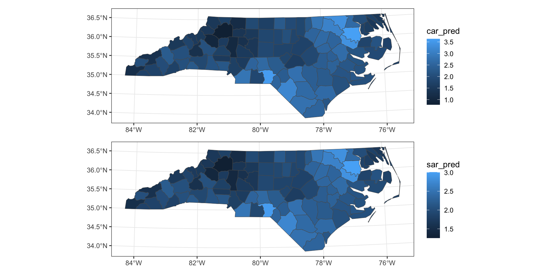
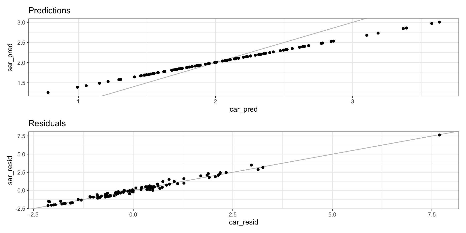
Predictions

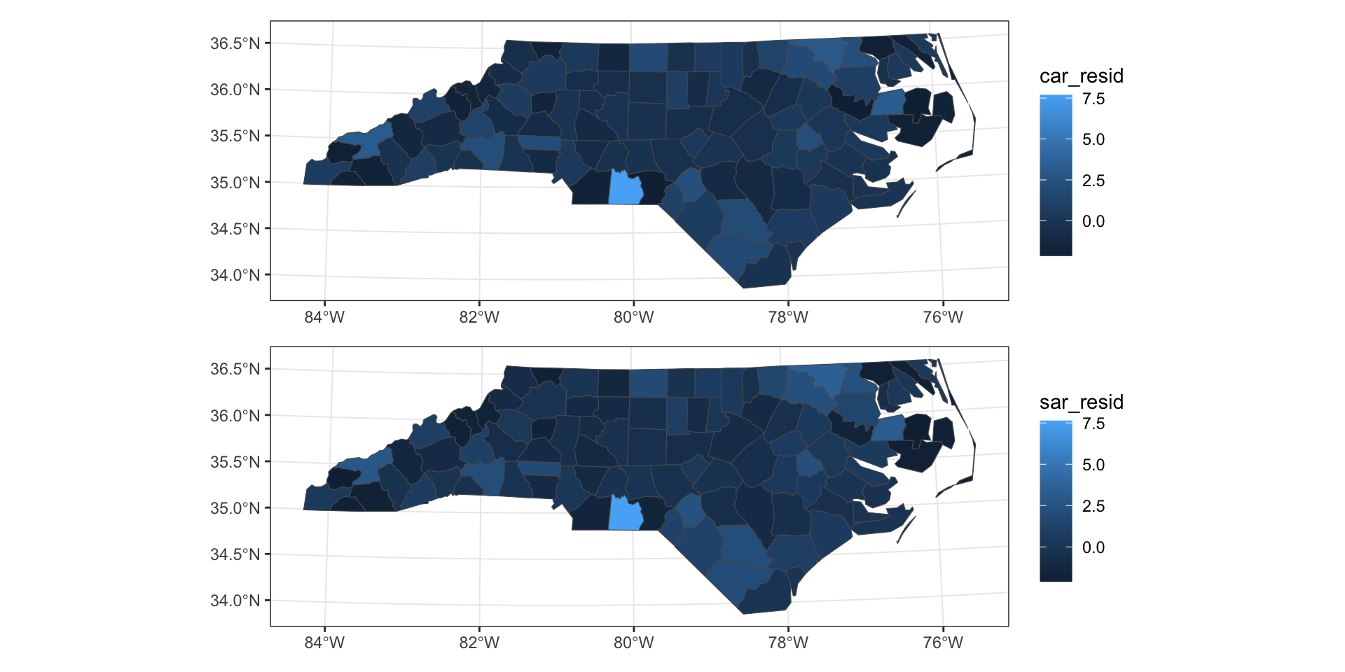
Residuals

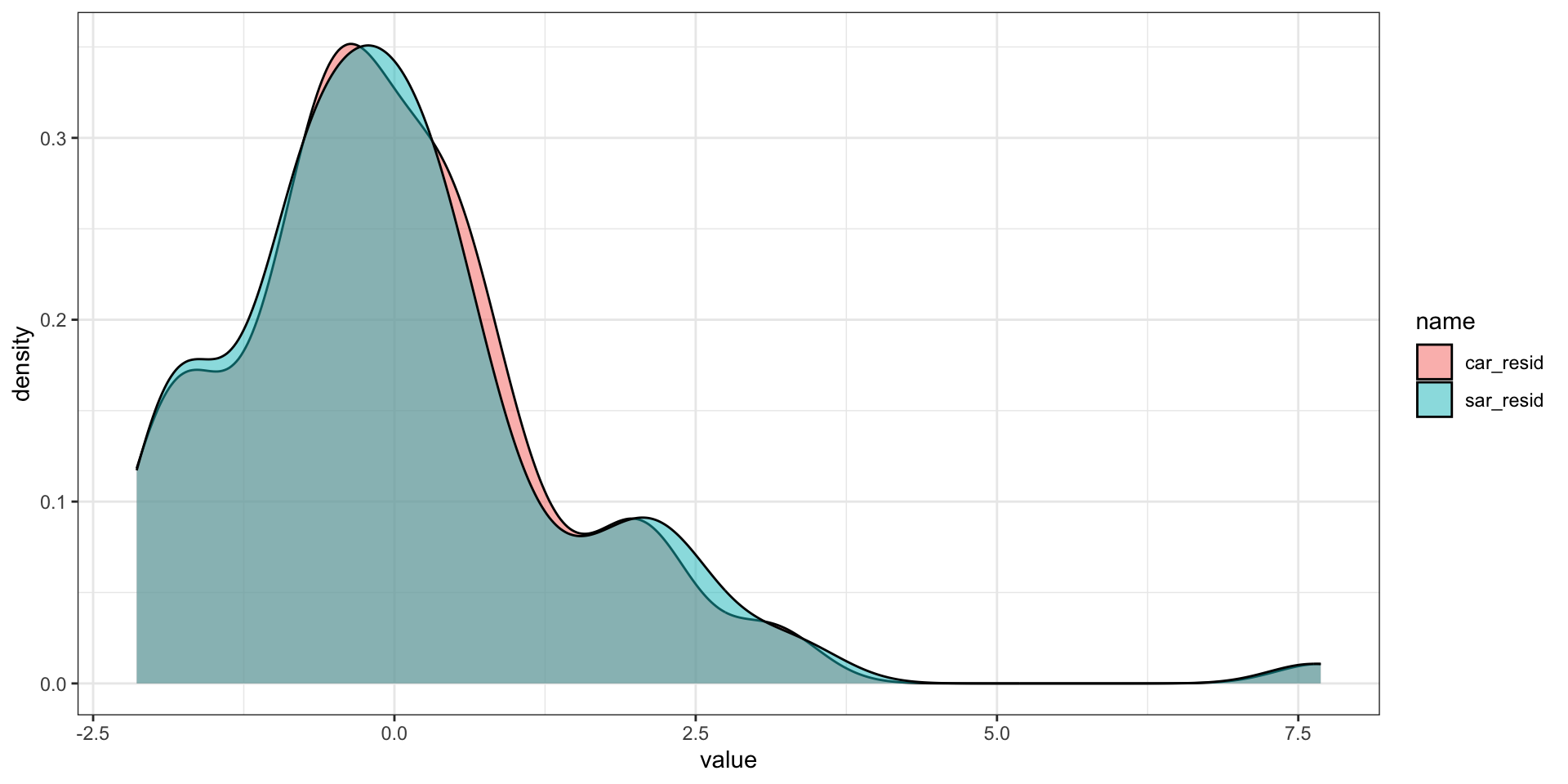
Residual distributions

Residual autocorrelation

spdep::moran.test(nc$car_resid, listW)

    Moran I test under randomisation

data:  nc$car_resid  
weights: listW    

Moran I statistic standard deviate =
-1.7952, p-value = 0.9637
alternative hypothesis: greater
sample estimates:
Moran I statistic       Expectation 
     -0.117449316      -0.010101010 
         Variance 
      0.003575538 

spdep::moran.test(nc$sar_resid, listW)

    Moran I test under randomisation

data:  nc$sar_resid  
weights: listW    

Moran I statistic standard deviate =
0.17958, p-value = 0.4287
alternative hypothesis: greater
sample estimates:
Moran I statistic       Expectation 
     0.0006769074     -0.0101010101 
         Variance 
     0.0036020941 

spdep::moran.test(nc$car_resid, listW, alternative = "two.sided")

    Moran I test under randomisation

data:  nc$car_resid  
weights: listW    

Moran I statistic standard deviate =
-1.7952, p-value = 0.07261
alternative hypothesis: two.sided
sample estimates:
Moran I statistic       Expectation 
     -0.117449316      -0.010101010 
         Variance 
      0.003575538 

spdep::moran.test(nc$sar_resid, listW, alternative = "two.sided")

    Moran I test under randomisation

data:  nc$sar_resid  
weights: listW    

Moran I statistic standard deviate =
0.17958, p-value = 0.8575
alternative hypothesis: two.sided
sample estimates:
Moran I statistic       Expectation 
     0.0006769074     -0.0101010101 
         Variance 
     0.0036020941 

Predicted vs Observed

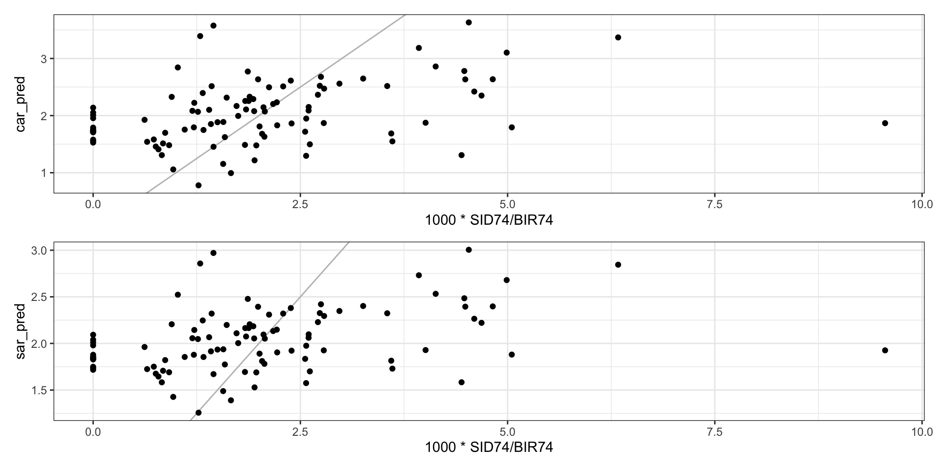
What’s wrong?

Comparing CAR vs SAR.

Transforming the data

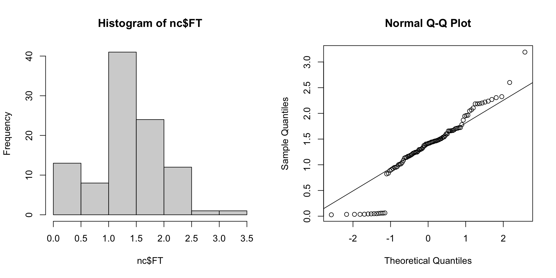
Freeman-Tukey’s transformation

This is the transformation used by Cressie and Road in Spatial Data Analysis of Regional Counts (1989).

\[ FT = \sqrt{1000} \left( \sqrt{\frac{SID74}{BIR74}} + \sqrt{\frac{SID74+1}{BIR74}} \right) \]

Other possibilities

nc = mutate(nc, 
  sqrt = sqrt(1000*(SID74+1)/BIR74),
  log  = log(1000*(SID74+1)/BIR74),
)

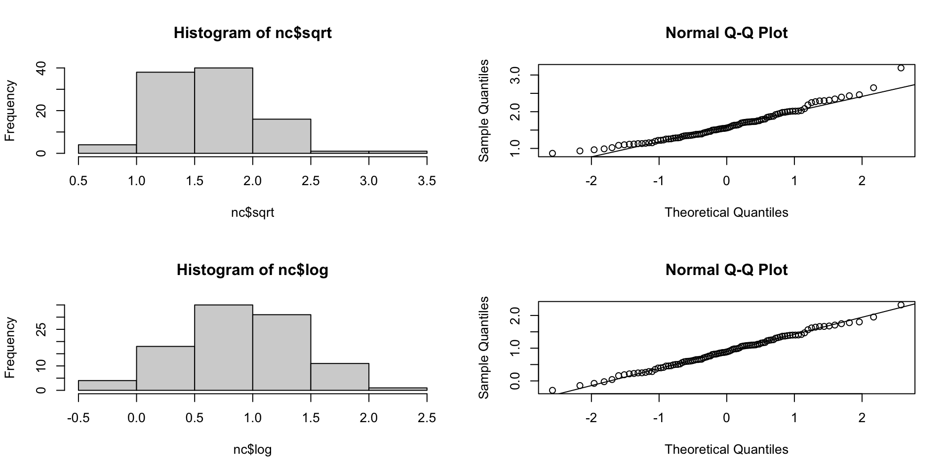
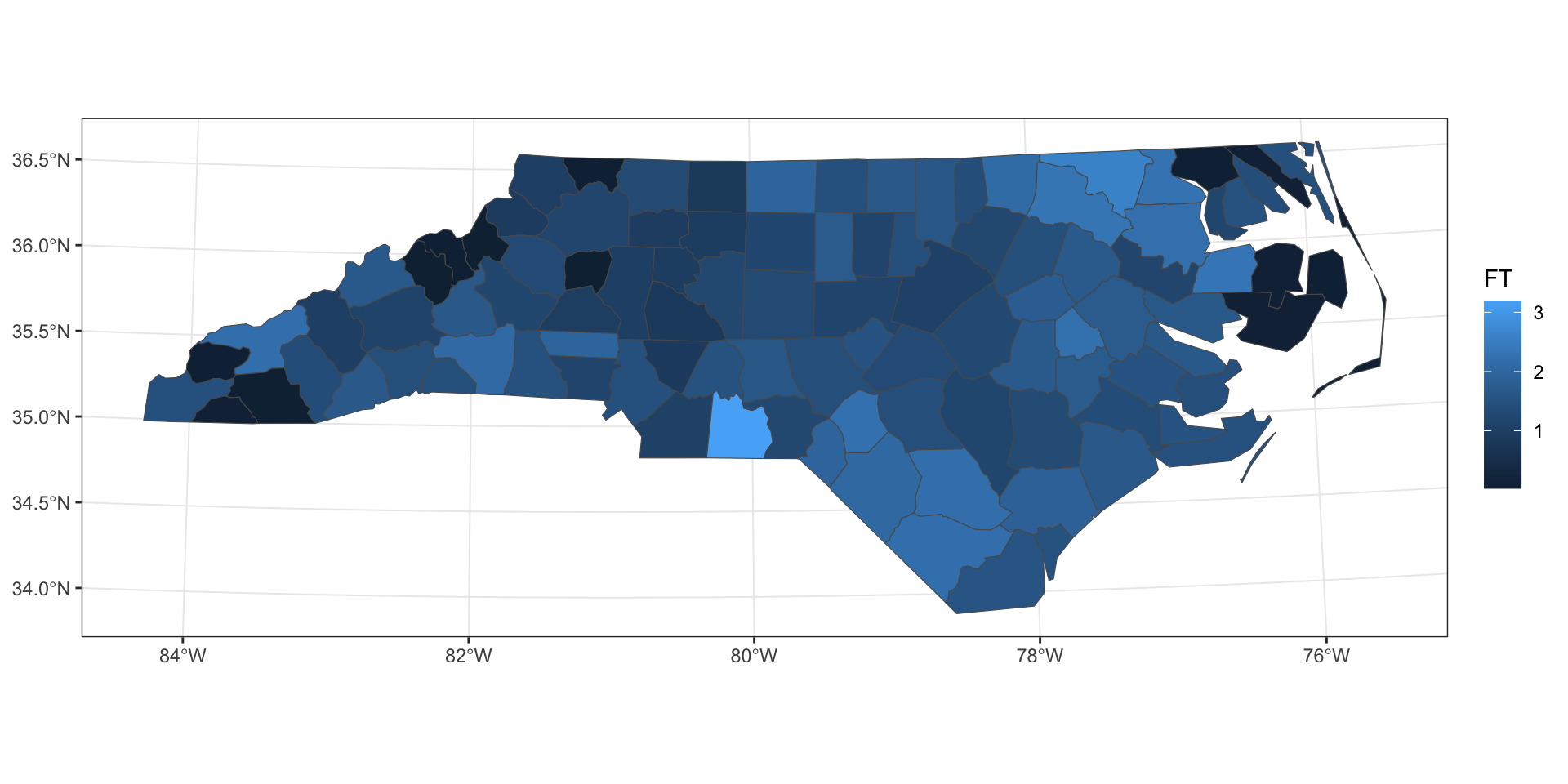
FT transformation

ggplot(nc) + geom_sf(aes(fill=FT))

spdep::moran.test(nc$FT, listW)

    Moran I test under randomisation

data:  nc$FT  
weights: listW    

Moran I statistic standard deviate = 3.664,
p-value = 0.0001242
alternative hypothesis: greater
sample estimates:
Moran I statistic       Expectation 
      0.216246481      -0.010101010 
         Variance 
      0.003816298 

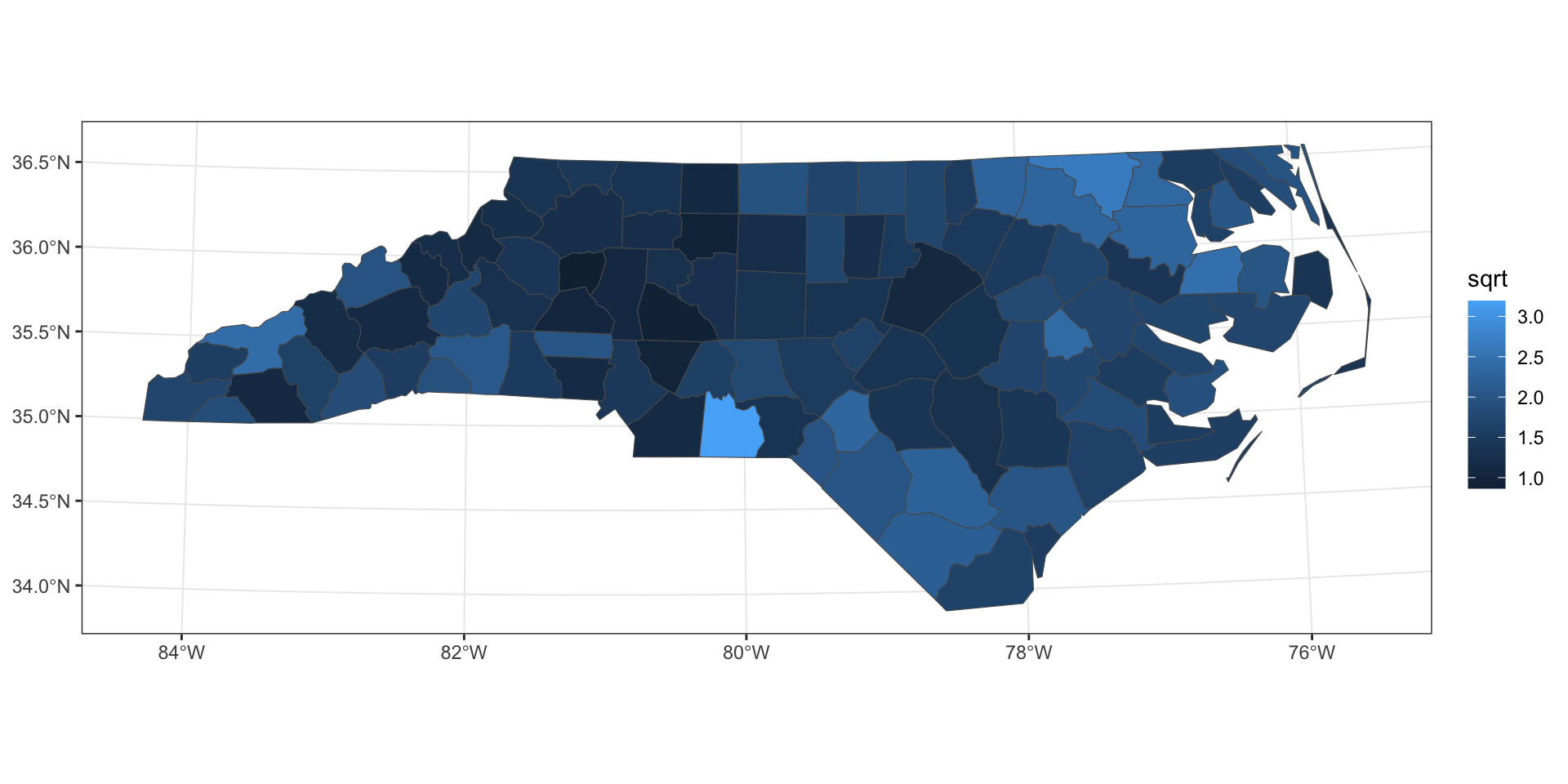
sqrt transformation

ggplot(nc) + geom_sf(aes(fill=sqrt))

spdep::moran.test(nc$sqrt, listW)

    Moran I test under randomisation

data:  nc$sqrt  
weights: listW    

Moran I statistic standard deviate = 4.5217,
p-value = 3.067e-06
alternative hypothesis: greater
sample estimates:
Moran I statistic       Expectation 
      0.268600322      -0.010101010 
         Variance 
      0.003798988 

log transformation

ggplot(nc) + geom_sf(aes(fill=log))

spdep::moran.test(nc$log, listW)

    Moran I test under randomisation

data:  nc$log  
weights: listW    

Moran I statistic standard deviate = 4.9895,
p-value = 3.027e-07
alternative hypothesis: greater
sample estimates:
Moran I statistic       Expectation 
      0.299245438      -0.010101010 
         Variance 
      0.003843927 

CAR Models

nc_car_ft   = spatialreg::spautolm(formula = FT ~ 1,   data = nc, listw = listW, family = "CAR") 
nc_car_sqrt = spatialreg::spautolm(formula = sqrt ~ 1, data = nc, listw = listW, family = "CAR")
nc_car_log  = spatialreg::spautolm(formula = log ~ 1,  data = nc, listw = listW, family = "CAR")

AIC(nc_car_ft)

[1] 192.1781

AIC(nc_car_sqrt)

[1] 100.8898

AIC(nc_car_log)

[1] 134.644

SAR Model

nc_sar_ft   = spatialreg::spautolm(formula = FT ~ 1,   data = nc, listw = listW, family = "SAR") 
nc_sar_sqrt = spatialreg::spautolm(formula = sqrt ~ 1, data = nc, listw = listW, family = "SAR")
nc_sar_log  = spatialreg::spautolm(formula = log ~ 1,  data = nc, listw = listW, family = "SAR")

AIC(nc_sar_ft)

[1] 191.9918

AIC(nc_sar_sqrt)

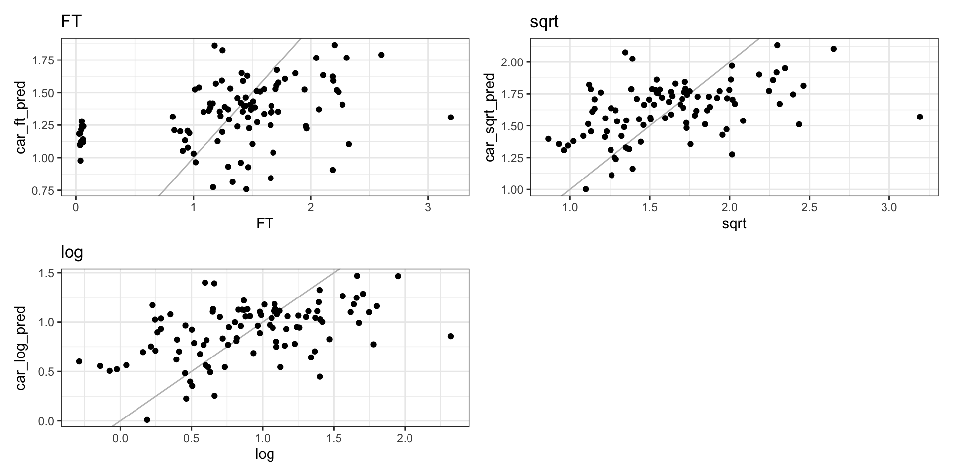
[1] 102.717

AIC(nc_sar_log)

[1] 137.4095

CAR predictions

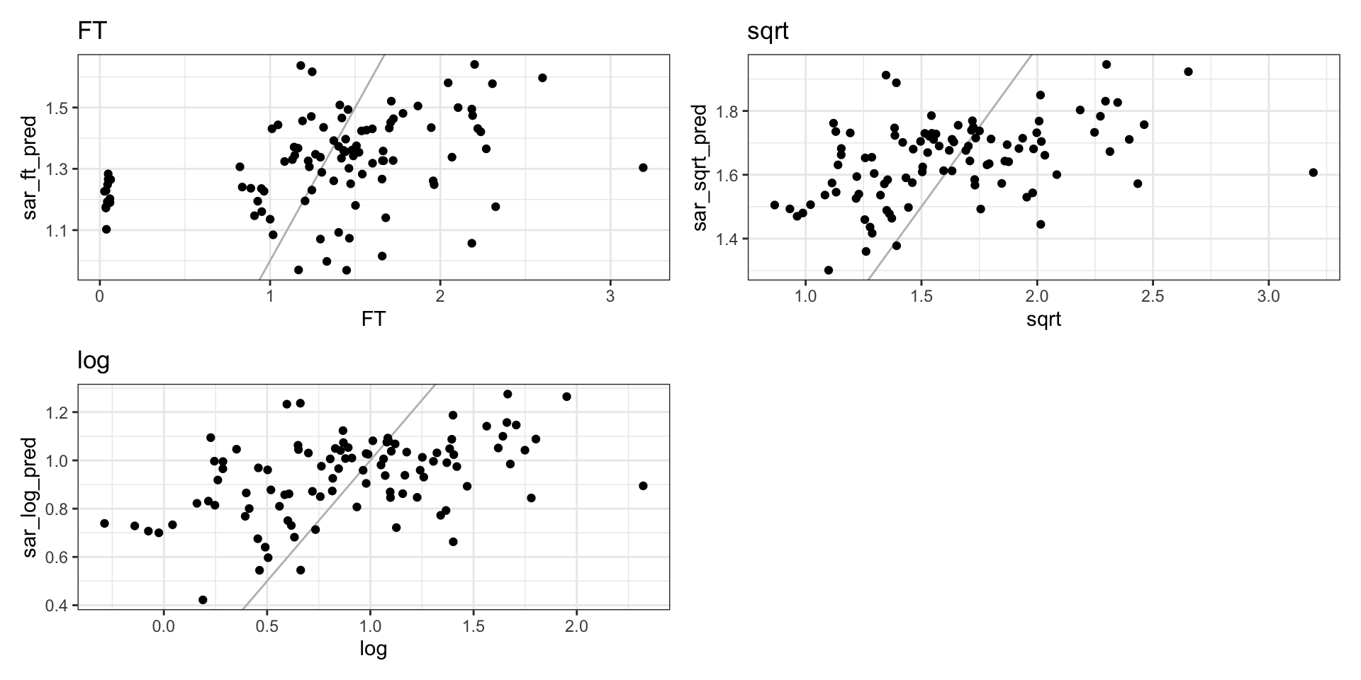
SAR predictions

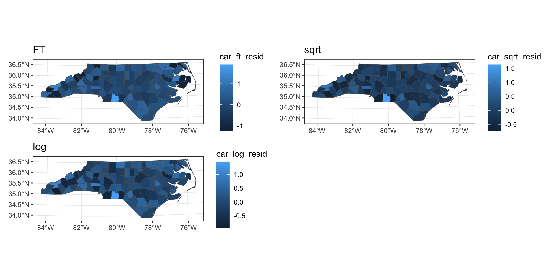
CAR residuals

SAR predictions

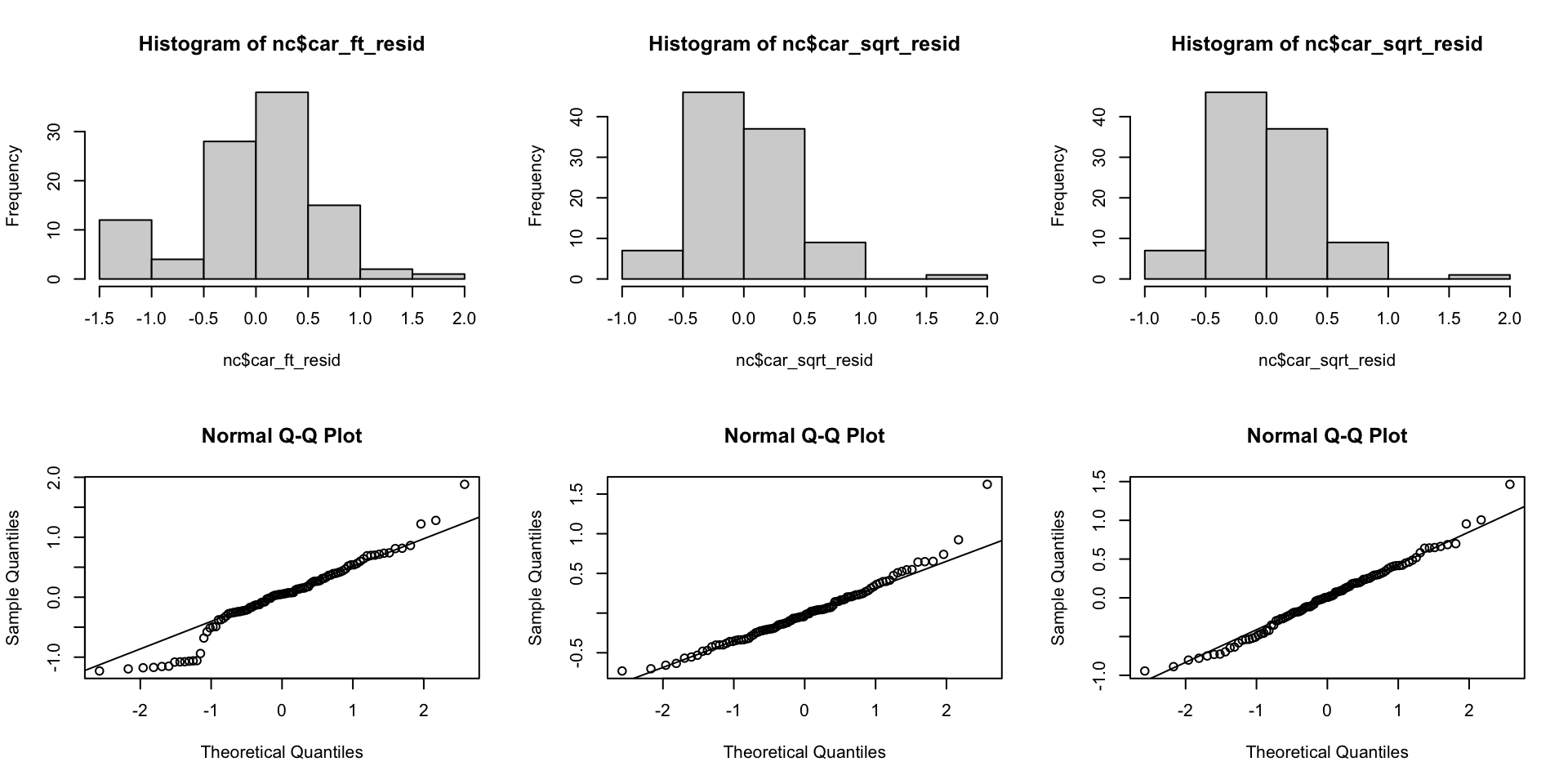
CAR residual distributions

SAR residual distributions

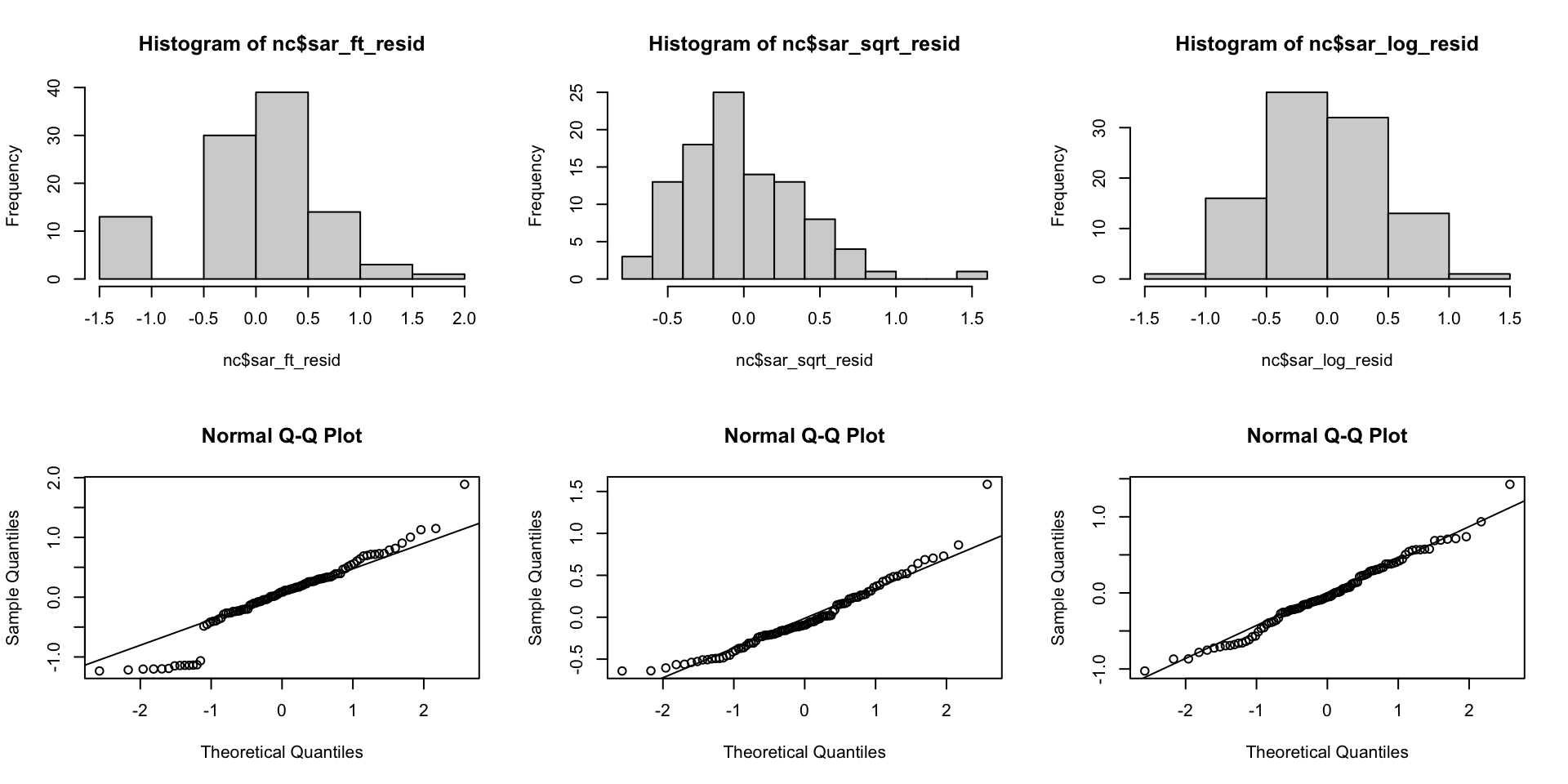
Residual spatial autocorrelation

spdep::moran.test(nc$car_sqrt_resid, listW)

    Moran I test under randomisation

data:  nc$car_sqrt_resid  
weights: listW    

Moran I statistic standard deviate =
-3.1196, p-value = 0.9991
alternative hypothesis: greater
sample estimates:
Moran I statistic       Expectation 
     -0.200890550      -0.010101010 
         Variance 
      0.003740354 

spdep::moran.test(nc$sar_sqrt_resid, listW)

    Moran I test under randomisation

data:  nc$sar_sqrt_resid  
weights: listW    

Moran I statistic standard deviate = -0.422,
p-value = 0.6635
alternative hypothesis: greater
sample estimates:
Moran I statistic       Expectation 
     -0.035976080      -0.010101010 
         Variance 
      0.003759585 

CAR & SAR with brms

brms CAR

b_car = brms::brm(
    1000*SID74/BIR74 ~ 1 + car(A), data=nc, data2=list(A=A),
    adapt_delta = 0.95,
    silent=2, refresh=0, iter=20000,
    cores = 4, backend = "cmdstanr"
)

Running MCMC with 4 parallel chains...

Chain 3 finished in 11.0 seconds.
Chain 2 finished in 11.7 seconds.
Chain 4 finished in 12.4 seconds.
Chain 1 finished in 12.7 seconds.

All 4 chains finished successfully.
Mean chain execution time: 12.0 seconds.
Total execution time: 12.8 seconds.

b_car

 Family: gaussian 
  Links: mu = identity; sigma = identity 
Formula: 1000 * SID74/BIR74 ~ 1 + car(A) 
   Data: nc (Number of observations: 100) 
  Draws: 4 chains, each with iter = 20000; warmup = 10000; thin = 1;
         total post-warmup draws = 40000

Correlation Structures:
      Estimate Est.Error l-95% CI u-95% CI Rhat
car       0.74      0.16     0.35     0.97 1.00
sdcar     2.73      0.44     1.67     3.40 1.01
      Bulk_ESS Tail_ESS
car       1159     2327
sdcar      492     1386

Population-Level Effects: 
          Estimate Est.Error l-95% CI u-95% CI
Intercept     2.09      0.32     1.45     2.73
          Rhat Bulk_ESS Tail_ESS
Intercept 1.01      594      679

Family Specific Parameters: 
      Estimate Est.Error l-95% CI u-95% CI Rhat
sigma     0.50      0.32     0.07     1.21 1.05
      Bulk_ESS Tail_ESS
sigma       87       18

Draws were sampled using sample(hmc). For each parameter, Bulk_ESS
and Tail_ESS are effective sample size measures, and Rhat is the potential
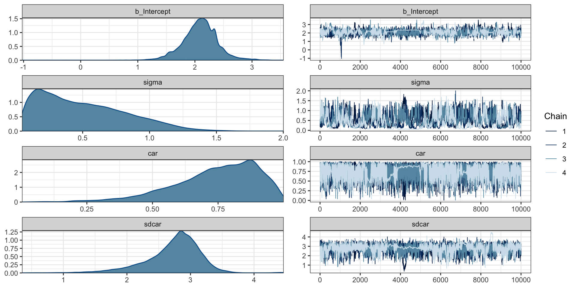
scale reduction factor on split chains (at convergence, Rhat = 1).

Diagnostics

plot(b_car)

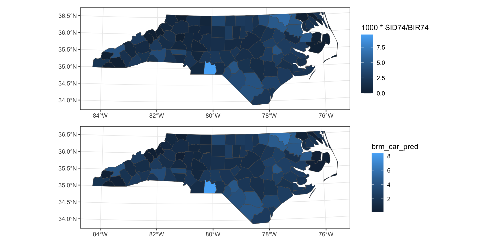
Predictions

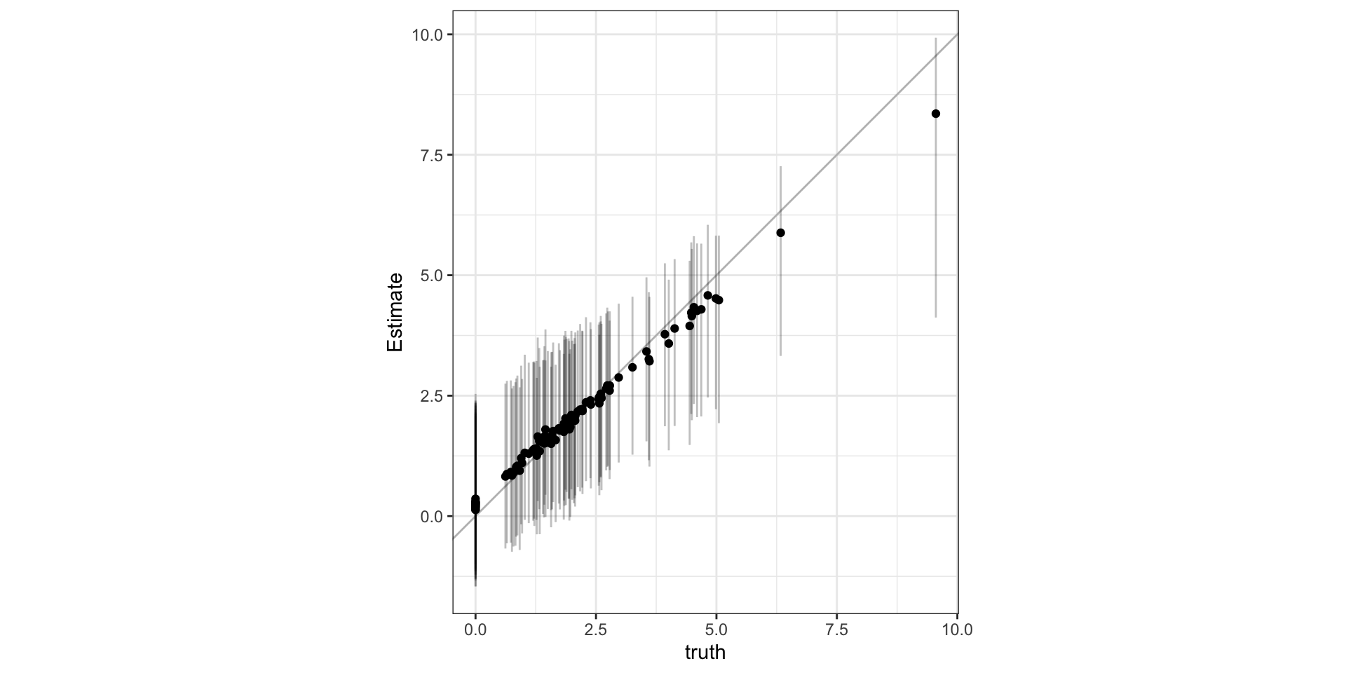
Observed vs predicted

ggplot(p, aes(x=truth, y=Estimate)) +
  geom_abline(intercept=0, slope=1, color="grey") +
  geom_point() +
  geom_errorbar(aes(ymin=Q2.5, ymax=Q97.5), alpha=0.25) +
  coord_fixed()

brms SAR

b_sar = brms::brm(
    1000*SID74/BIR74 ~ 1 + sar(listW), data=nc, data2=list(listW=listW),
    silent=2, refresh=0, iter=4000,
    cores = 4, backend = "cmdstanr"
)

Running MCMC with 4 parallel chains...

Chain 3 finished in 2.9 seconds.
Chain 4 finished in 2.8 seconds.
Chain 1 finished in 2.9 seconds.
Chain 2 finished in 2.8 seconds.

All 4 chains finished successfully.
Mean chain execution time: 2.9 seconds.
Total execution time: 3.2 seconds.

b_sar

 Family: gaussian 
  Links: mu = identity; sigma = identity 
Formula: 1000 * SID74/BIR74 ~ 1 + sar(listW) 
   Data: nc (Number of observations: 100) 
  Draws: 4 chains, each with iter = 4000; warmup = 2000; thin = 1;
         total post-warmup draws = 8000

Correlation Structures:
       Estimate Est.Error l-95% CI u-95% CI Rhat
lagsar     0.06      0.02     0.02     0.10 1.00
       Bulk_ESS Tail_ESS
lagsar     3128     3877

Population-Level Effects: 
          Estimate Est.Error l-95% CI u-95% CI
Intercept     1.42      0.26     0.91     1.94
          Rhat Bulk_ESS Tail_ESS
Intercept 1.00     2911     3789

Family Specific Parameters: 
      Estimate Est.Error l-95% CI u-95% CI Rhat
sigma     1.52      0.11     1.33     1.75 1.00
      Bulk_ESS Tail_ESS
sigma     5052     4845

Draws were sampled using sample(hmc). For each parameter, Bulk_ESS
and Tail_ESS are effective sample size measures, and Rhat is the potential
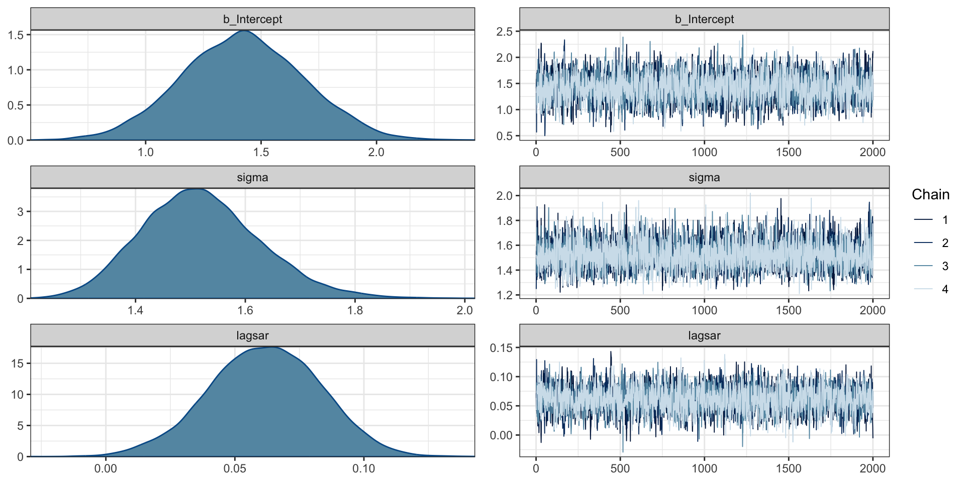
scale reduction factor on split chains (at convergence, Rhat = 1).

Diagnostics

plot(b_sar)

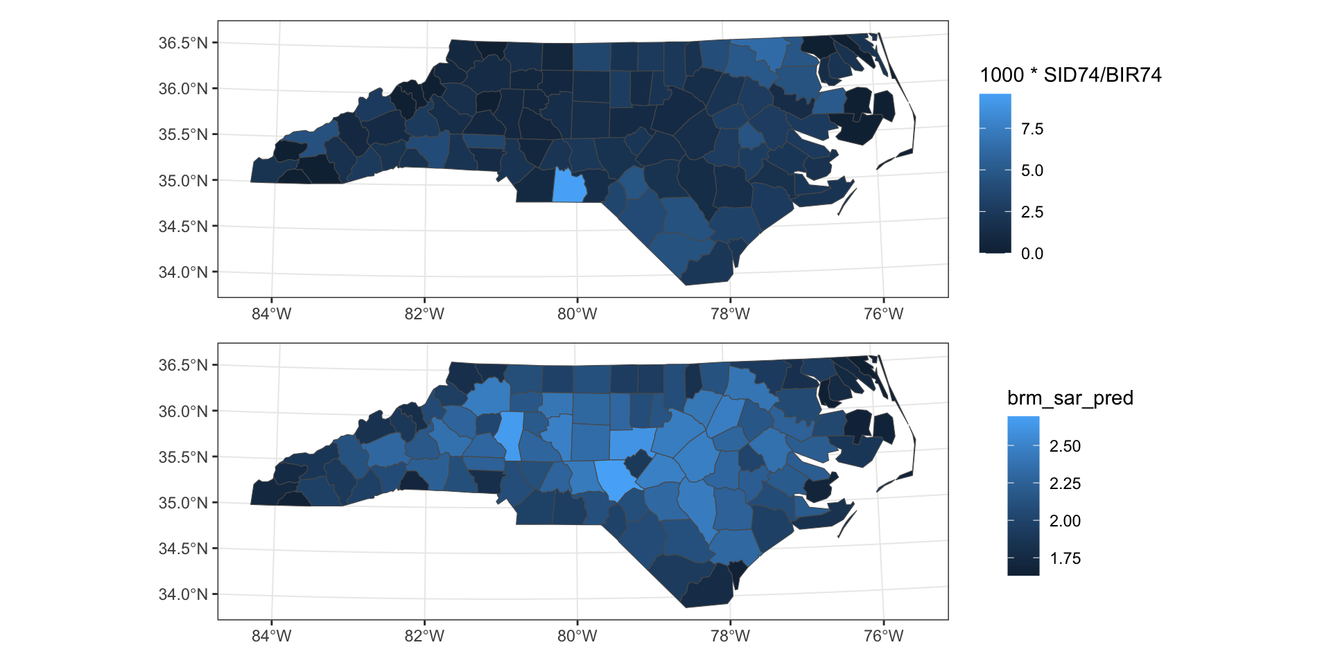
Predictions

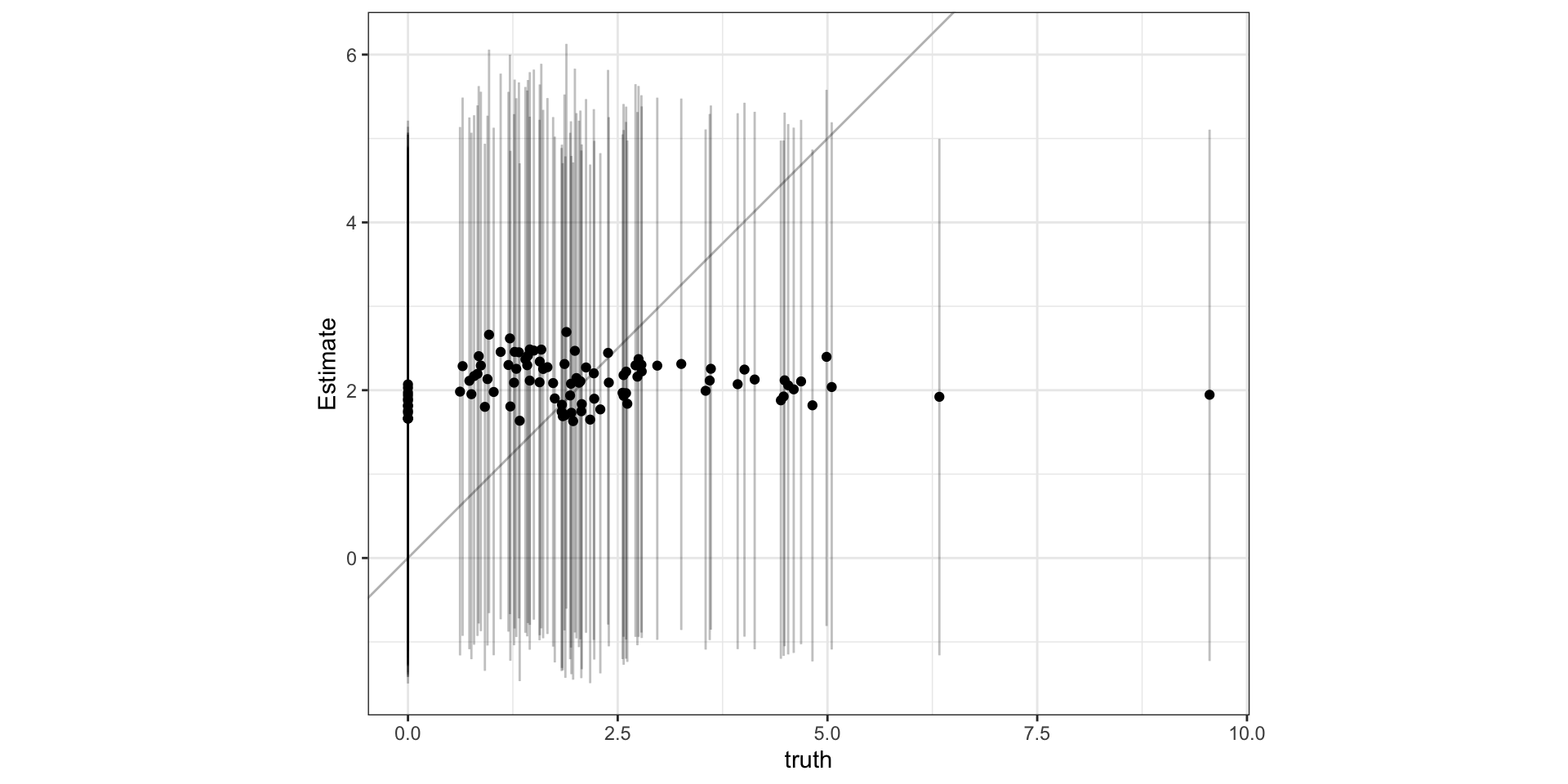
Observed vs predicted

ggplot(p, aes(x=truth, y=Estimate)) +
  geom_abline(intercept=0, slope=1, color="grey") +
  geom_point() +
  geom_errorbar(aes(ymin=Q2.5, ymax=Q97.5), alpha=0.25) +
  coord_fixed()

Brief Aside - CAR & SAR precision matrices

\[ \Sigma_{SAR} = (\boldsymbol{I}-\phi \boldsymbol{D}^{-1} \, \boldsymbol{A})^{-1} \sigma^2 \, \boldsymbol{D}^{-1} \left((\boldsymbol{I}-\phi \boldsymbol{D}^{-1} \, \boldsymbol{A})^{-1}\right)^t \]

\[ \begin{aligned} \Sigma^{-1}_{SAR} &= \left( (\boldsymbol{I}-\phi \boldsymbol{D}^{-1} \, \boldsymbol{A})^{-1} \sigma^2 \, \boldsymbol{D}^{-1} \left((\boldsymbol{I}-\phi \boldsymbol{D}^{-1} \, \boldsymbol{A})^{-1}\right)^t \right)^{-1} \\ &= \left( \left( (\boldsymbol{I}-\phi \boldsymbol{D}^{-1} \, \boldsymbol{A})^{-1}\right)^t\right)^{-1} \frac{1}{\sigma^2} \, \boldsymbol{D} ~ (\boldsymbol{I}-\phi \boldsymbol{D}^{-1} \, \boldsymbol{A}) \\ &= \frac{1}{\sigma^2} \, (\boldsymbol{I}-\phi \boldsymbol{D}^{-1} \, \boldsymbol{A})^t ~ \boldsymbol{D} ~ (\boldsymbol{I}-\phi \boldsymbol{D}^{-1} \, \boldsymbol{A}) \\ \end{aligned} \]

\[ \Sigma^{-1}_{CAR} = \frac{1}{\sigma^2} \, (\boldsymbol{D}- \phi \boldsymbol{A}) \]