      [,1] [,2] [,3] [,4] [,5] [,6] [,7] [,8] [,9] [,10] [,11] [,12]
 [1,]    0    1    0    0    0    0    0    0    0     0     0     0
 [2,]    1    0    1    0    0    0    0    0    0     0     0     0
 [3,]    0    1    0    0    0    0    0    0    0     1     0     0
 [4,]    0    0    0    0    0    0    1    0    0     0     0     0
 [5,]    0    0    0    0    0    1    0    0    1     0     0     0
 [6,]    0    0    0    0    1    0    0    1    0     0     0     0
 [7,]    0    0    0    1    0    0    0    1    0     0     0     0
 [8,]    0    0    0    0    0    1    1    0    0     0     0     0
 [9,]    0    0    0    0    1    0    0    0    0     0     0     0
[10,]    0    0    1    0    0    0    0    0    0     0     0     1
[11,]    0    0    0    0    0    0    0    0    0     0     0     1
[12,] 0 0 0 0 0 0 0 0 0 1 1 0Models for areal data
Lecture 19
areal / lattice data
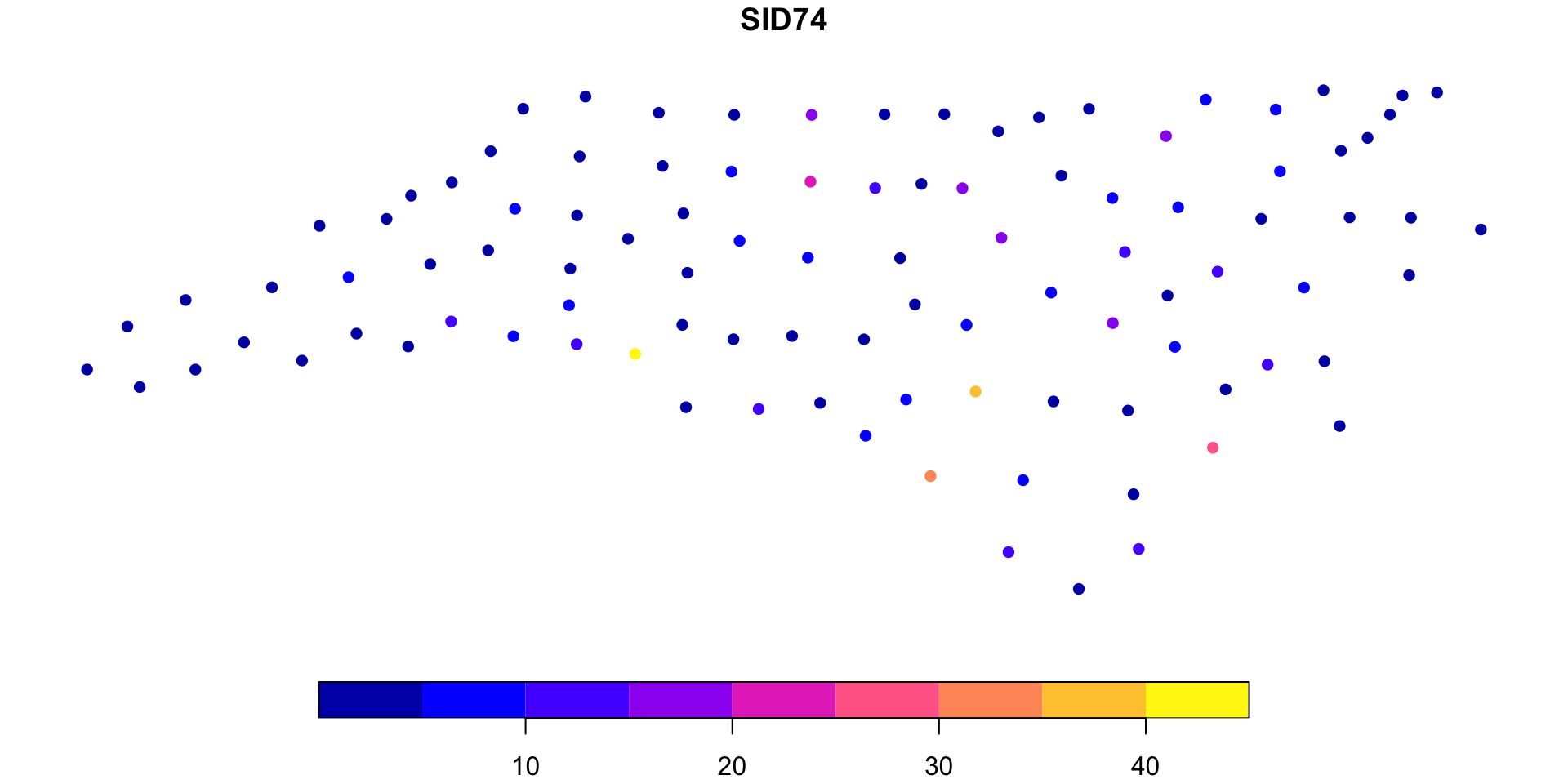
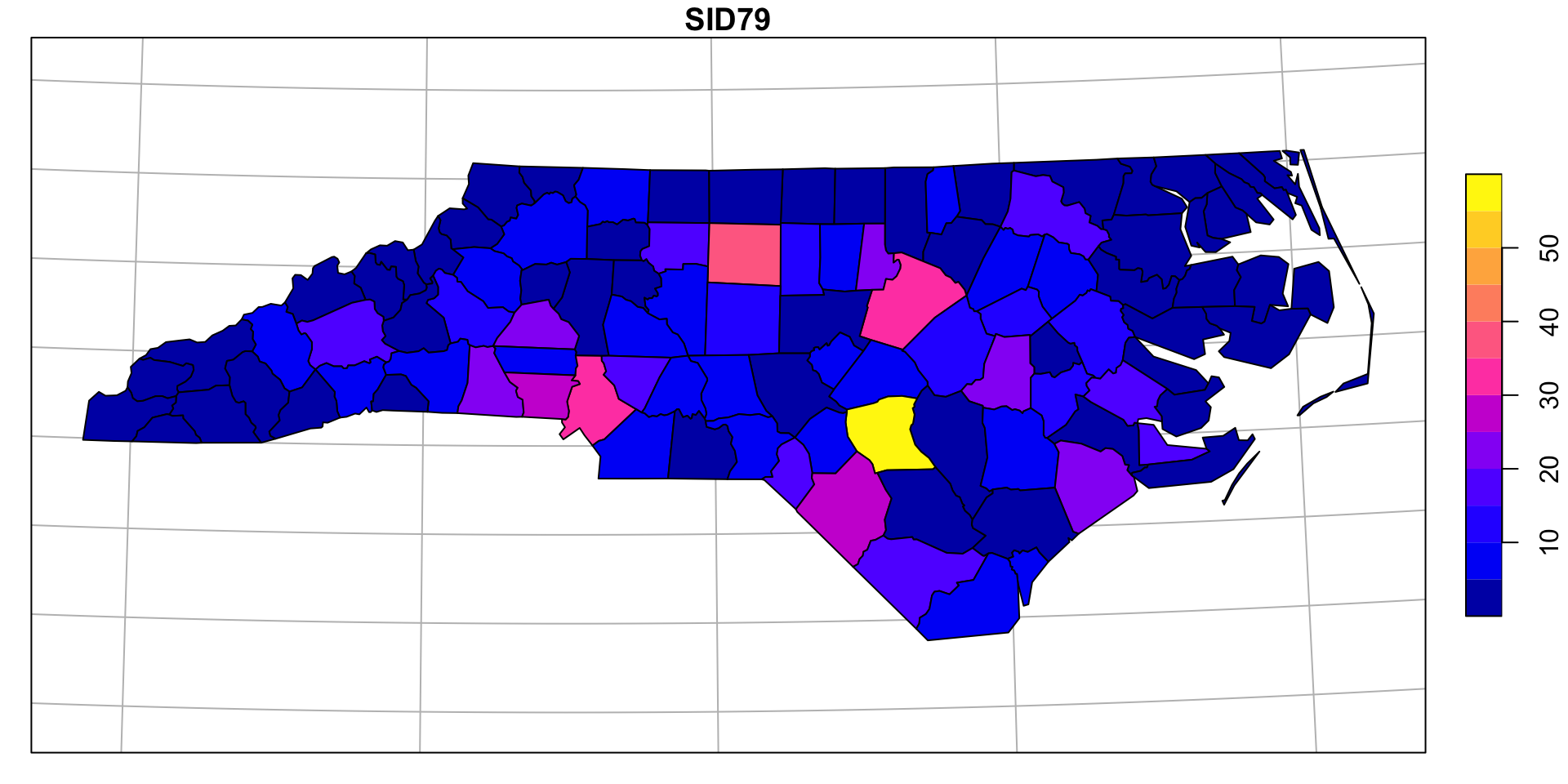
Example - NC SIDS
Adjacency Matrix
Normalized spatial weight matrix
normalize_weights = function(w) {
  w = 1*w
  diag(w) = 0
  rs = rowSums(w)
  rs[rs == 0] = 1
  w/rs
}
normalize_weights( st_touches(nc[1:12,], sparse=FALSE) )
[,1] [,2] [,3] [,4] [,5] [,6] [,7] [,8] [,9] [,10] [,11] [,12]
[1,] 0.0 1.0 0.0 0.0 0.0 0.0 0.0 0.0 0.0 0.0 0.0 0.0
[2,] 0.5 0.0 0.5 0.0 0.0 0.0 0.0 0.0 0.0 0.0 0.0 0.0
[3,] 0.0 0.5 0.0 0.0 0.0 0.0 0.0 0.0 0.0 0.5 0.0 0.0
[4,] 0.0 0.0 0.0 0.0 0.0 0.0 1.0 0.0 0.0 0.0 0.0 0.0
[5,] 0.0 0.0 0.0 0.0 0.0 0.5 0.0 0.0 0.5 0.0 0.0 0.0
[6,] 0.0 0.0 0.0 0.0 0.5 0.0 0.0 0.5 0.0 0.0 0.0 0.0
[7,] 0.0 0.0 0.0 0.5 0.0 0.0 0.0 0.5 0.0 0.0 0.0 0.0
[8,] 0.0 0.0 0.0 0.0 0.0 0.5 0.5 0.0 0.0 0.0 0.0 0.0
[9,] 0.0 0.0 0.0 0.0 1.0 0.0 0.0 0.0 0.0 0.0 0.0 0.0
[10,] 0.0 0.0 0.5 0.0 0.0 0.0 0.0 0.0 0.0 0.0 0.0 0.5
[11,] 0.0 0.0 0.0 0.0 0.0 0.0 0.0 0.0 0.0 0.0 0.0 1.0
[12,] 0.0 0.0 0.0 0.0 0.0 0.0 0.0 0.0 0.0 0.5 0.5 0.0EDA - Moran’s I
If we have observations at \(n\) spatial locations \((s_1, \ldots s_n)\)
\[ I = \frac{n}{\sum_{i=1}^n \sum_{j=1}^n w_{ij}} \frac{\sum_{i=1}^n \sum_{j=1}^n w_{ij} \big(y(s_i)-\bar{y}\big)\big(y(s_j)-\bar{y}\big)}{\sum_{i=1}^n \big(y(s_i) - \bar{y}\big)^2} \] where \(\boldsymbol{w}\) is a spatial weights matrix.
Some properties of Moran’s I when there is no spatial autocorrelation / dependence:
\(E(I) = -1 / (n-1)\)
\(Var(I) = (\text{Something ugly but closed form})- E(I)^2\)
\(\underset{n\to\infty}{\lim} \frac{I - E(I)}{\sqrt{Var(I)}} \sim N(0,1)\) (via the CLT)
NC SIDS & Moran’s I
Lets start by using a normalized spatial weight matrix for \(\boldsymbol{w}\) (basedd on shared county borders).
EDA - Geary’s C
Like Moran’s I, if we have observations at \(n\) spatial locations \((s_1, \ldots s_n)\)
\[ C = \frac{n-1}{2\sum_{i=1}^n \sum_{j=1}^n w_{ij}} \frac{\sum_{i=1}^n \sum_{j=1}^n w_{ij} \big(y(s_i)-y(s_j)\big)^2}{\sum_{i=1}^n \big(y(s_i) - \bar{y}\big)^2} \] where \(\boldsymbol{w}\) is a spatial weights matrix.
Some properties of Geary’s C:
- \(0 < C < 2\)
- If \(C \approx 1\) then no spatial autocorrelation
- If \(C > 1\) then negative spatial autocorrelation
- If \(C < 1\) then positive spatial autocorrelation
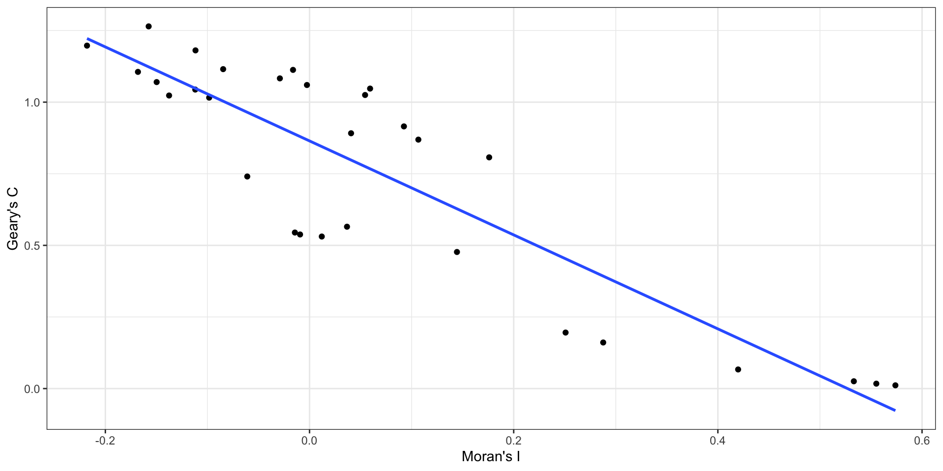
- Geary’s C is inversely related to Moran’s I
NC SIDS & Geary’s C
Again using an normalized adjacency matrix for \(\boldsymbol{w}\) (shared county borders).
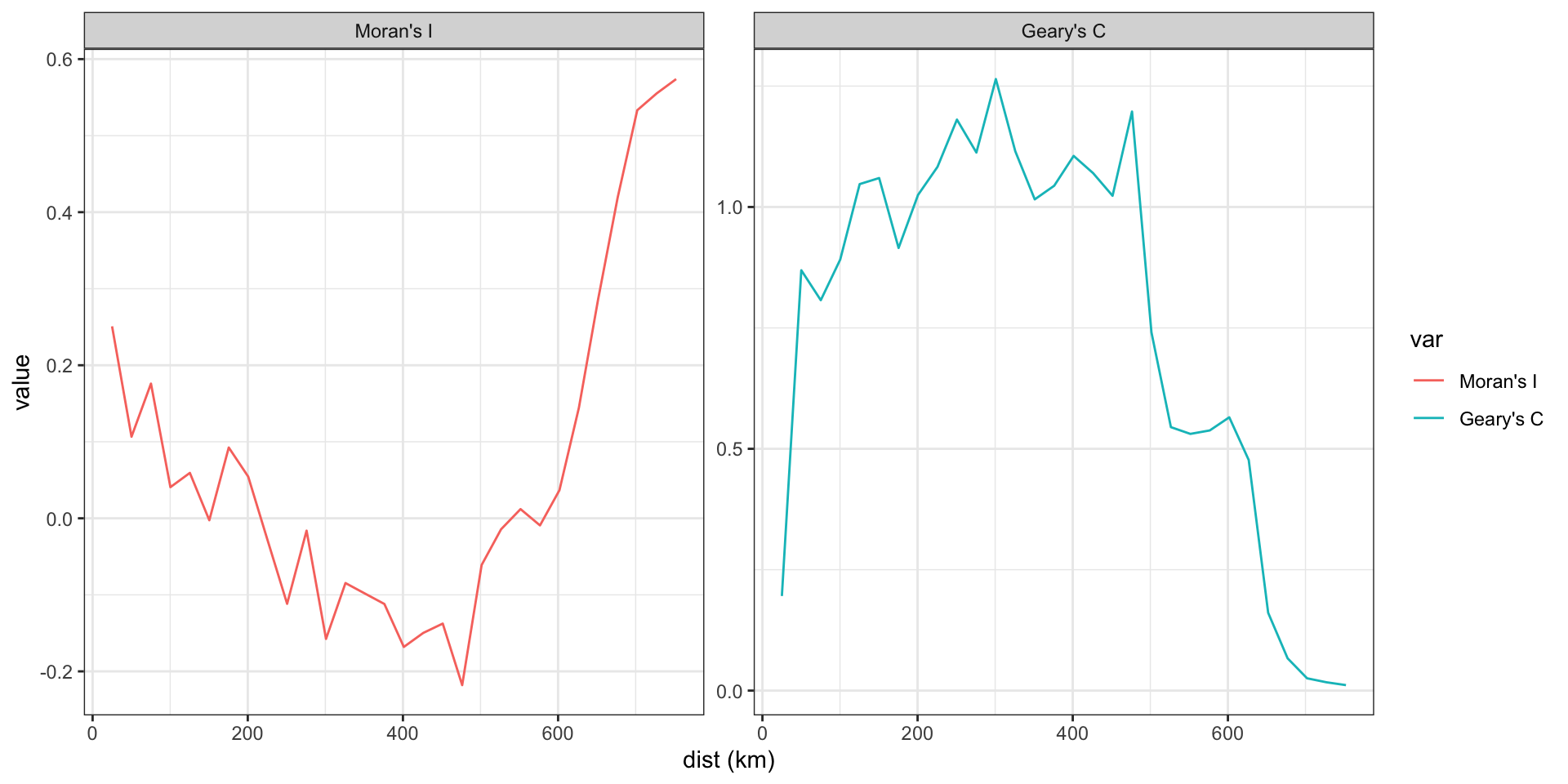
Spatial Correlogram
Here we are defining adjacency based on the centroid being within a given distance,
Autoregressive Models
AR Models - Time
Lets return to the simplest case, an \(AR(1)\) process
\[ y_t = \delta + \phi \, y_{t-1} + w_t \]
where \(w_t \sim N(0,\sigma^2_w)\) and \(|\phi| < 1\), then
\[ \begin{aligned} E(y_t) &= \frac{\delta}{1-\phi} \\ Var(y_t) &= \frac{\sigma^2}{1-\phi} \\ \rho(h) &= \phi^{h} \\ \gamma(h) &= \phi^h \frac{\sigma^2}{1-\phi} \end{aligned} \]
AR Models - Time - Joint Distribution
Previously we saw that an \(AR(1)\) model can be represented using a multivariate normal distribution
\[ \begin{pmatrix} y_1 \\ y_2 \\ \vdots \\ y_n \end{pmatrix} \sim N \begin{pmatrix} \frac{\delta}{1-\phi} \begin{pmatrix}1\\ 1\\ \vdots\\ 1\end{pmatrix},~ \frac{\sigma^2}{1-\phi} \begin{pmatrix} 1 & \phi & \cdots & \phi^{n-1} \\ \phi & 1 & \cdots & \phi^{n-2} \\ \vdots & \vdots & \ddots & \vdots \\ \phi^{n-1} & \phi^{n-2} & \cdots & 1 \\ \end{pmatrix} \end{pmatrix} \]
In writing down the likelihood we also saw that an \(AR(1)\) is 1st order Markovian,
\[ \begin{aligned} f(y_1, \ldots, y_n) &= f(y_1) \, f(y_2 \mid y_1) \, f(y_3 \mid y_2,y_1) \,\cdots\, f(y_n|y_{n-1},y_{n-2},\ldots,y_1) \\ &= f(y_1) \, f(y_2 \mid y_1) \, f(y_3 \mid y_2) \,\cdots\, f(y_n \mid y_{n-1}) \end{aligned} \]
Alternative Definitions for \(y_t\)
\[ y_t = \delta + \phi \, y_{t-1} + w_t \]
vs.
\[ y_t\mid y_{t-1} \sim N(\delta + \phi \, y_{t-1},~\sigma^2) \]
In the case of time, both of these definitions result in the same multivariate distribution for \(\boldsymbol{y}\) given on the previous slide.
AR in Space

Even in the simplest spatial case there is no clear / unique ordering,
\[ \begin{aligned} f\big(y(s_1), \ldots, y(s_{10})\big) &= f\big(y(s_1)\big) \, f\big(y(s_2) \mid y(s_1)\big) \, \cdots \, f\big(y(s_{10}\mid y(s_{9}),y(s_{8}),\ldots,y(s_1)\big) \\ &= f\big(y(s_{10})\big) \, f\big(y(s_9) \mid y(s_{10})\big) \, \cdots \, f\big(y(s_{1}\mid y(s_{2}),y(s_{3}),\ldots,y(s_{10})\big) \\ &= ~? \end{aligned} \]
Instead we need to think about things in terms of their neighbors / neighborhoods. We define \(N(s_i)\) to be the set of neighbors of location \(s_i\).
If we define the neighborhood based on “touching” then \(N(s_3) = \{s_2, s_4\}\)
If we use distance within 2 units then \(N(s_3) = \{s_1,s_2,s_3,s_4\}\)
Defining the Spatial AR model
Here we will consider a simple average of neighboring observations, just like with the temporal AR model we have two options in terms of defining the autoregressive process,
- Simultaneous Autogressve (SAR) \[ y(s) = \delta + \phi \frac{1}{|N(s)|}\sum_{s' \in N(s)} y(s') + N(0,\sigma^2) \]
- Conditional Autoregressive (CAR) \[ y(s) \mid y(-s) \sim N\left(\delta + \phi \frac{1}{|N(s)|}\sum_{s' \in N(s)} y(s'),~ \sigma^2 \right) \]
Simultaneous Autogressve (SAR)
Using \[ y(s) = \phi \frac{1}{|N(s)|}\sum_{s' \in N(s)} y(s') + N(0,\sigma^2) \] we want to find the distribution of \(\boldsymbol{y} = \Big(y(s_1),\, y(s_2),\,\ldots,\,y(s_n)\Big)^t\).
First we can define a weight matrix \(\boldsymbol{W}\) where \[ \{\boldsymbol{W}\}_{ij} = \begin{cases} 1/|N(s_i)| & \text{if $j \in N(s_i)$} \\ 0 & \text{otherwise} \end{cases} \] then we can write \(\boldsymbol{y}\) as follows, \[ \boldsymbol{y} = \phi \, \boldsymbol{W} \, \boldsymbol{y} + \boldsymbol{\epsilon} \] where \[ \boldsymbol{\epsilon} \sim N(0,\sigma^2 \, \boldsymbol{I}) \]
A toy example

Back to SAR
\[ \boldsymbol{y} = \phi \, \boldsymbol{W} \, \boldsymbol{y} + \boldsymbol{\epsilon} \]
Conditional Autogressve (CAR)
This is a bit trickier, in the case of the temporal AR process we actually went from joint distribution \(\to\) conditional distributions (which we were then able to simplify).
Since we don’t have a natural ordering we can’t get away with this (at least not easily).
Going the other way, conditional distributions \(\to\) joint distribution is difficult because it is possible to specify conditional distributions that lead to an improper joint distribution.
Brooks’ Lemma
For sets of observations \(\boldsymbol{x}\) and \(\boldsymbol{y}\) where \(p(x) > 0~~\forall ~ x\in\boldsymbol{x}\) and \(p(y) > 0~~\forall ~ y\in\boldsymbol{y}\) then
\[ \begin{aligned} \frac{p(\boldsymbol{y})}{p(\boldsymbol{x})} &= \prod_{i=1}^n \frac{p(y_i \mid y_1,\ldots,y_{i-1},x_{i+1},\ldots,x_n)}{p(x_i \mid y_1,\ldots,y_{i-1},x_{i+1},\ldots,x_n)} \\ &= \prod_{i=1}^n \frac{p(y_i \mid x_1,\ldots,x_{i-1},y_{i+1},\ldots,y_n)}{p(x_i \mid x_1,\ldots,x_{i-1},y_{i+1},\ldots,y_n)} \\ \end{aligned} \]
A simplified example
Let \(\boldsymbol{y} = (y_1,y_2)\) and \(\boldsymbol{x} = (x_1,x_2)\) then we can derive Brook’s Lemma for this case,
\[ \begin{aligned} p (y_1,y_2) &= p(y_1 \mid y_2) p(y_2) \\ &= p(y_1 \mid y_2) \frac{p(y_2 \mid x_1)}{p(x_1 \mid y_2)} p(x_1) \\ & = \frac{p(y_1 \mid y_2)}{p(x_1 \mid y_2)} p(y_2 \mid x_1) \, p(x_1) \\ & = \frac{p(y_1 \mid y_2)}{p(x_1 \mid y_2)} p(y_2 \mid x_1) \, p(x_1) \left(\frac{p(x_2 \mid x_1)}{p(x_2 \mid x_1)}\right) \\ & = \frac{p(y_1 \mid y_2)}{p(x_1 \mid y_2)} \frac{p(y_2 \mid x_1)}{p(x_2 \mid x_1)} \, p(x_1,x_2) \\ \end{aligned} \]
This is just a derivation of Brook’s lemma for \(\boldsymbol{y} = (y_1,y_2)\) and \(\boldsymbol{x} = (x_1,x_2)\).
\[ \begin{aligned} p (y_1,y_2) & = \frac{p(y_1 \mid y_2)}{p(x_1 \mid y_2)} \frac{p(y_2 \mid x_1)}{p(x_2 \mid x_1)} \, p(x_1,x_2) \\ \\ \frac{p (y_1,y_2) }{p(x_1,x_2)} & = \frac{p(y_1 \mid y_2)}{p(x_1 \mid y_2)} \frac{p(y_2 \mid x_1)}{p(x_2 \mid x_1)} \end{aligned} \]
From which we can generalize for \(n=3\),
\[ \begin{aligned} \frac{p(y_1,y_2,y_3)}{p(x_1,x_2,x_3)} = \frac{p(y_1 \mid y_2,y_3)}{p(x_1 \mid y_2,y_3)} \frac{p(y_2 \mid x_1,y_3)}{p(x_2 \mid x_1,y_3} \frac{p(y_3 \mid x_1,x_2)}{p(x_3 \mid x_1,x_2)} \end{aligned} \] and so on.
Utility?
Lets repeat that last example but consider the case where \(\boldsymbol{y} = (y_1,y_2)\) but now we let \(\boldsymbol{x} = (y_1=0,y_2=0)\)
\[ \begin{aligned} \frac{p (y_1,y_2) }{p(x_1,x_2)} &= \frac{p (y_1,y_2) }{p(y_1=0,y_2=0)} \end{aligned} \]
\[ \begin{aligned} p(y_1,y_2) &= \frac{p(y_1 \mid y_2)}{p(y_1=0 \mid y_2)} \frac{p(y_2 \mid y_1=0)}{p(y_2=0 \mid y_1=0)} ~ p(y_1=0,y_2=0) \end{aligned} \]
\[ \begin{aligned} p(y_1,y_2) &\propto \frac{p(y_1 \mid y_2) ~ p(y_2 \mid y_1=0) }{ p(y_1=0 \mid y_2)} \\ &\propto \frac{p(y_2 \mid y_1) ~ p(y_1 \mid y_2=0) }{ p(y_2=0 \mid y_1)} \end{aligned} \]
As applied to a simple CAR
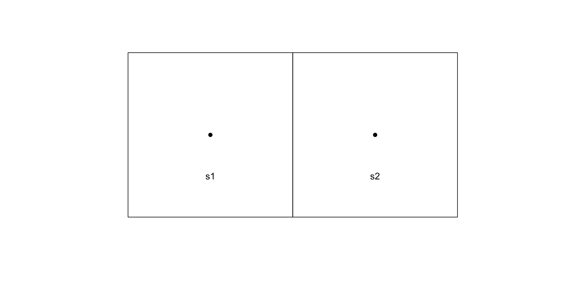
\[ \begin{aligned} y(s_1)\mid y(s_2) \sim N(\phi W_{12}\, y(s_2),\, \sigma^2) \\ y(s_2)\mid y(s_1) \sim N(\phi W_{21}\, y(s_1),\, \sigma^2) \end{aligned} \]
\[ \begin{aligned} p\big(y(s_1),y(s_2)\big) &\propto \frac{p\big(y(s_1) \mid y(s_2)\big) ~ p\big(y(s_2) \mid y(s_1)=0\big)}{p\big(y(s_1)=0 \mid y(s_2)\big)}\\ &\propto \frac{ \exp\left(-\frac{1}{2\sigma^2}\left(y(s_1)-\phi \, W_{12} \, y(s_2)\right)^2\right) \exp\left(-\frac{1}{2\sigma^2}\left(y(s_2)-\phi \, W_{21} \, 0\right)^2\right) }{ \exp\left(-\frac{1}{2\sigma^2}\left(0-\phi W_{12} y(s_2)\right)^2 \right) }\\ &\propto \exp\left(-\frac{1}{2\sigma^2}\left(\left(y(s_1)-\phi \, W_{12} \, y(s_2)\right)^2 + y(s_2)^2- (\phi W_{21} y(s_2))^2\right)\right) \\ &\propto \exp\left(-\frac{1}{2\sigma^2}\left(y(s_1)^2-\phi \, W_{12} \, y(s_1)\,y(s_2) -\phi \, W_{21} \, y(s_1)\,y(s_2) + y(s_2)^2\right)\right) \\ &\propto \exp\left(-\frac{1}{2\sigma^2} (\boldsymbol{y}-0) \begin{pmatrix} 1 & -\phi W_{12} \\ -\phi W_{21} & 1 \end{pmatrix} (\boldsymbol{y}-0)^{t} \right) \end{aligned} \]
Implications for \(\boldsymbol{y}\)
\[ \boldsymbol{\mu} = 0 \]
\[ \begin{aligned} \boldsymbol{\Sigma}^{-1} &= \frac{1}{\sigma^2} \begin{pmatrix} 1 & -\phi W_{12} \\ -\phi W_{21} & 1 \end{pmatrix} \\ &= \frac{1}{\sigma^2}(\boldsymbol{I} - \phi \, \boldsymbol{W}) \end{aligned} \]
\[ \boldsymbol{\Sigma} = \sigma^2(\boldsymbol{I} - \phi \, \boldsymbol{W})^{-1} \]
we can then conclude that for \(\boldsymbol{y} = (y(s_1),~y(s_2))^t\),
\[ \boldsymbol{y} \sim N\left( \boldsymbol{0}, ~ \sigma^2 (\boldsymbol{I} - \phi \, \boldsymbol{W})^{-1} \right) \]
which generalizes for all mean 0 CAR models.
General Proof
Let \(\boldsymbol{y} = (y(s_1),\ldots,y(s_n))\) and \(\boldsymbol{0} = (y(s_1) = 0, \ldots, y(s_n)=0)\) then by Brook’s lemma,
\[ \begin{aligned} \frac{p(\boldsymbol{y})}{p(\boldsymbol{0})} &= \prod_{i=1}^n \frac{p(y_i \mid y_1,\ldots,y_{i-1},0_{i+1},\ldots,0_{n})}{p(0_i \mid y_1,\ldots,y_{i-1},0_{i+1},\ldots,0_{n})} = \prod_{i=1}^n \frac{ \exp\left(-\frac{1}{2\sigma^2} \left(y_i - \phi \sum_{j<i} W_{ij} \, y_j - \phi \sum_{j>i} 0_j \right)^2 \right) }{ \exp\left(-\frac{1}{2\sigma^2} \left(0_i - \phi \sum_{j<i} W_{ij} \, y_j - \phi \sum_{j>i} 0_j \right)^2 \right) } \\ &= \exp\left(-\frac{1}{2\sigma^2} \sum_{i=1}^n \left(y_i - \phi \sum_{j<i} W_{ij} \, y_j\right)^2 + \frac{1}{2\sigma^2} \sum_{i=1}^n \left( \phi \sum_{j<i} W_{ij} \, y_j \right)^2 \right) \\ &= \exp\left(-\frac{1}{2\sigma^2} \sum_{i=1}^n y_i^2 - 2 \phi y_i \,\sum_{j<i} W_{ij} \, y_j \right) \\ &= \exp\left(-\frac{1}{2\sigma^2} \sum_{i=1}^n y_i^2 - \phi \sum_{i=1}^n \sum_{j=1}^n y_i \, W_{ij} \, y_j \right) \quad \mathit{\big(\text{if } W_{ij} = W_{ji}\big)} \\ &= \exp\left(-\frac{1}{2\sigma^2} (\boldsymbol{y}-0)^t (\boldsymbol{I} - \phi \boldsymbol{W}) (\boldsymbol{y}-0) \right) \end{aligned} \]
CAR vs SAR
- Simultaneous Autogressve (SAR)
\[ y(s) = \phi \sum_{s'} W_{s\;s'} \, y(s') + \epsilon \]
\[ \boldsymbol{y} \sim N(0,~\sigma^2 \, ((\boldsymbol{I}-\phi \boldsymbol{W})^{-1}) ((\boldsymbol{I}-\phi \boldsymbol{W})^{-1})^t )\]
- Conditional Autoregressive (CAR)
\[ y(s) \mid y(-s) \sim N\left(\sum_{s'} W_{s\;s'} \, y(s'),~ \sigma^2 \right) \]
\[ \boldsymbol{y} \sim N(0,~\sigma^2 \, (\boldsymbol{I}-\phi \boldsymbol{W})^{-1})\]
Generalizations
Adopting different weight matrices \((\boldsymbol{W})\)
Between SAR and CAR model we move to a generic weight matrix definition (beyond average of nearest neighbors)
In time we varied \(p\) in the \(AR(p)\) model, in space we adjust the weight matrix.
In general having a symmetric W is helpful, but not required
More complex Variance (beyond \(\sigma^2 \, I\))
\(\sigma^2\) can be a vector (differences between areal locations)
i.e. since areal data tends to be aggregated - adjust variance based on sample size
i.e. scale based on the number of neighbors
Some specific generalizations
Generally speaking we want to work with a scaled / normalized version of the weight matrix, \[ W_{ij}/W_{i\boldsymbol{\cdot}} \]
When \(W\) is derived from an adjacency matrix, \(\boldsymbol{A}\), we can express this as \[ \boldsymbol{W} = \boldsymbol{D}^{-1} \boldsymbol{A} \] where \(\boldsymbol{D}^{-1} = \text{diag}(1/|N(s_i)|)\).
We can also allow \(\sigma^2\) to vary between locations, we can define this as \(\boldsymbol{D}_{\sigma^2} = \text{diag}(\sigma^2_i)\) and most often we use \[ \boldsymbol{D}_{\sigma^2}^{-1} = \text{diag}\left(\frac{\sigma^2}{|N(s_i)|}\right) = \sigma^2 \boldsymbol{D}^{-1}. \]
Revised SAR Model
- Formula Model \[ y(s_i) = X_{i\cdot}\beta + \phi \sum_{j=1}^n D^{-1}_{jj} \, A_{ij} \, \big(y(s_j) - X_{j\cdot}\beta\big) + \epsilon_i \] \[ \boldsymbol{\epsilon} \sim N(\boldsymbol{0},\,\boldsymbol{D}_{\sigma^2}^{-1}) = N(\boldsymbol{0},\, \sigma^2 \boldsymbol{D}^{-1}) \]
- Joint Model \[ \boldsymbol{y} = \boldsymbol{X}\boldsymbol{\beta} + \phi \boldsymbol{D}^{-1} \boldsymbol{A} ~\big(\boldsymbol{y}-\boldsymbol{X}\boldsymbol{\beta}\big) + \boldsymbol{\epsilon} \]
\[ \boldsymbol{y} \sim N\left(\boldsymbol{X}\boldsymbol{\beta}, (\boldsymbol{I} - \phi \boldsymbol{D}^{-1} \boldsymbol{A})^{-1} \sigma^2 \boldsymbol{D}^{-1} \big((\boldsymbol{I} - \phi \boldsymbol{D}^{-1} \boldsymbol{A})^{-1}\big)^t \right) \]
Revised CAR Model
- Conditional Model \[ y(s_i) \mid y_{-s_i} \sim N\left(X_{i\cdot}\beta + \phi\sum_{j=1}^n \frac{W_{ij}}{D_{ii}} ~ \big(y(s_j)-X_{j\cdot}\beta\big),~ \sigma^2 D^{-1}_{ii} \right) \]
- Joint Model
\[ \boldsymbol{y} \sim N(\boldsymbol{X}\boldsymbol{\beta},~\Sigma_{CAR}) \]
\[ \begin{aligned} \Sigma_{CAR} &= (\boldsymbol{D}_{\sigma} \, (\boldsymbol{I}-\phi \boldsymbol{D}^{-1}\boldsymbol{A}))^{-1} \\ &= (1/\sigma^2 \boldsymbol{D} \, (\boldsymbol{I}-\phi \boldsymbol{D}^{-1}\boldsymbol{A}))^{-1} \\ &= (1/\sigma^2 (\boldsymbol{D}-\phi \boldsymbol{A}))^{-1} \\ &= \sigma^2(\boldsymbol{D}-\phi \boldsymbol{A})^{-1} \end{aligned} \]
Toy CAR Example
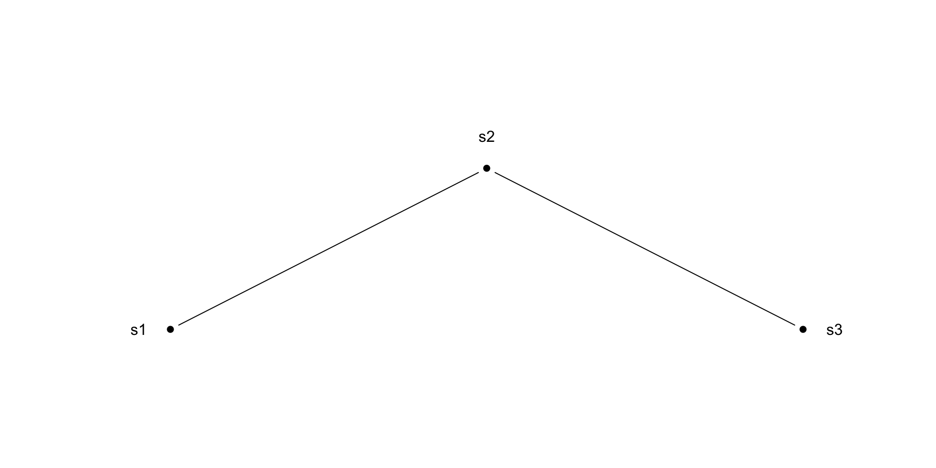
\[ \boldsymbol{A} = \begin{pmatrix} 0 & 1 & 0 \\ 1 & 0 & 1 \\ 0 & 1 & 0 \end{pmatrix} \qquad\qquad \boldsymbol{D} = \begin{pmatrix} 1 & 0 & 0 \\ 0 & 2 & 0 \\ 0 & 0 & 1 \end{pmatrix} \]
\[ \boldsymbol{\Sigma} = \sigma^2 \, (\boldsymbol{D} - \phi \, \boldsymbol{W}) = \sigma^2~\begin{pmatrix} 1 & -\phi & 0 \\ -\phi & 2 & -\phi \\ 0 & -\phi & 1 \end{pmatrix}^{-1} \]
When does \(\Sigma\) exist?
check_sigma = function(phi) {
  Sigma_inv = matrix(c(1,-phi,0,-phi,2,-phi,0,-phi,1), ncol=3, byrow=TRUE)
  solve(Sigma_inv)
}

check_sigma(phi=0)
[,1] [,2] [,3]
[1,] 1 0.0 0
[2,] 0 0.5 0
[3,] 0 0.0 1 [,1] [,2] [,3]
[1,] 1.1666667 0.3333333 0.1666667
[2,] 0.3333333 0.6666667 0.3333333
[3,] 0.1666667 0.3333333 1.1666667 [,1] [,2] [,3]
[1,] 1.28125 -0.46875 0.28125
[2,] -0.46875 0.78125 -0.46875
[3,] 0.28125 -0.46875 1.28125Error in solve.default(Sigma_inv): Lapack routine dgesv: system is exactly singular: U[3,3] = 0Error in solve.default(Sigma_inv): Lapack routine dgesv: system is exactly singular: U[3,3] = 0 [,1] [,2] [,3]
[1,] -0.6363636 -1.363636 -1.6363636
[2,] -1.3636364 -1.136364 -1.3636364
[3,] -1.6363636 -1.363636 -0.6363636 [,1] [,2] [,3]
[1,] -0.6363636 1.363636 -1.6363636
[2,] 1.3636364 -1.136364 1.3636364
[3,] -1.6363636 1.363636 -0.6363636When is \(\Sigma\) positive semidefinite?
check_sigma_pd = function(phi) {
  Sigma_inv = matrix(c(1,-phi,0,-phi,2,-phi,0,-phi,1), ncol=3, byrow=TRUE)
  chol(solve(Sigma_inv))
}

check_sigma_pd(phi=0)
[,1] [,2] [,3]
[1,] 1 0.0000000 0
[2,] 0 0.7071068 0
[3,] 0 0.0000000 1 [,1] [,2] [,3]
[1,] 1.080123 0.3086067 0.1543033
[2,] 0.000000 0.7559289 0.3779645
[3,] 0.000000 0.0000000 1.0000000 [,1] [,2] [,3]
[1,] 1.131923 -0.4141182 0.2484709
[2,] 0.000000 0.7808688 -0.4685213
[3,] 0.000000 0.0000000 1.0000000Error in solve.default(Sigma_inv): Lapack routine dgesv: system is exactly singular: U[3,3] = 0Error in solve.default(Sigma_inv): Lapack routine dgesv: system is exactly singular: U[3,3] = 0Error in chol.default(solve(Sigma_inv)): the leading minor of order 1 is not positive definiteError in chol.default(solve(Sigma_inv)): the leading minor of order 1 is not positive definiteConclusions
Generally speaking just like the AR(1) model for time series we require that \(|\phi| < 1\) for the CAR model to be proper.
These results for \(\phi\) also apply in the context where \(\sigma^2_i\) is constant across locations, i.e. \[ \boldsymbol{\Sigma} = \big(\sigma^2 \, (\boldsymbol{I}-\phi \boldsymbol{D}^{-1}\boldsymbol{A})\big)^{-1} \]
As a side note, the special case where \(\phi=1\) is known as an intrinsic autoregressive (IAR) model and they are popular as an improper prior for spatial random effects. An additional sum constraint is necessary for identifiability \[\sum_{i=1}^n y(s_i) = 0\]
Sta 344 - Fall 2022
