Covariance Functions

Lecture 16

Dr. Colin Rundel

sta344 package

Basics

The package is based on the course organizartion and can be installed with,

remotes::install_github("sta344-fa22/sta344")

collects all of the utility functions from the host scripts (e.g. util-crps.R, fix_pred_draw.R, etc.)

library(sta344)
ls("package:sta344")

 [1] "avg_temp"            "calc_crps"           "cond_predict"       
 [4] "emp_semivariogram"   "epred_draws_fix"     "exp_cov"            
 [7] "exp_sv"              "gpglm"               "gplm"               
[10] "linear_cov"          "matern_cov"          "normalize_weights"  
[13] "nugget_cov"          "periodic_cov"        "pow_exp_cov"        
[16] "pow_exp_sv"          "predicted_draws_fix" "residual_draws_fix" 
[19] "rmvnorm"             "rquad_cov"           "sphere_cov"         
[22] "sq_exp_cov"          "sq_exp_sv"           "strip_attrs"

From last time

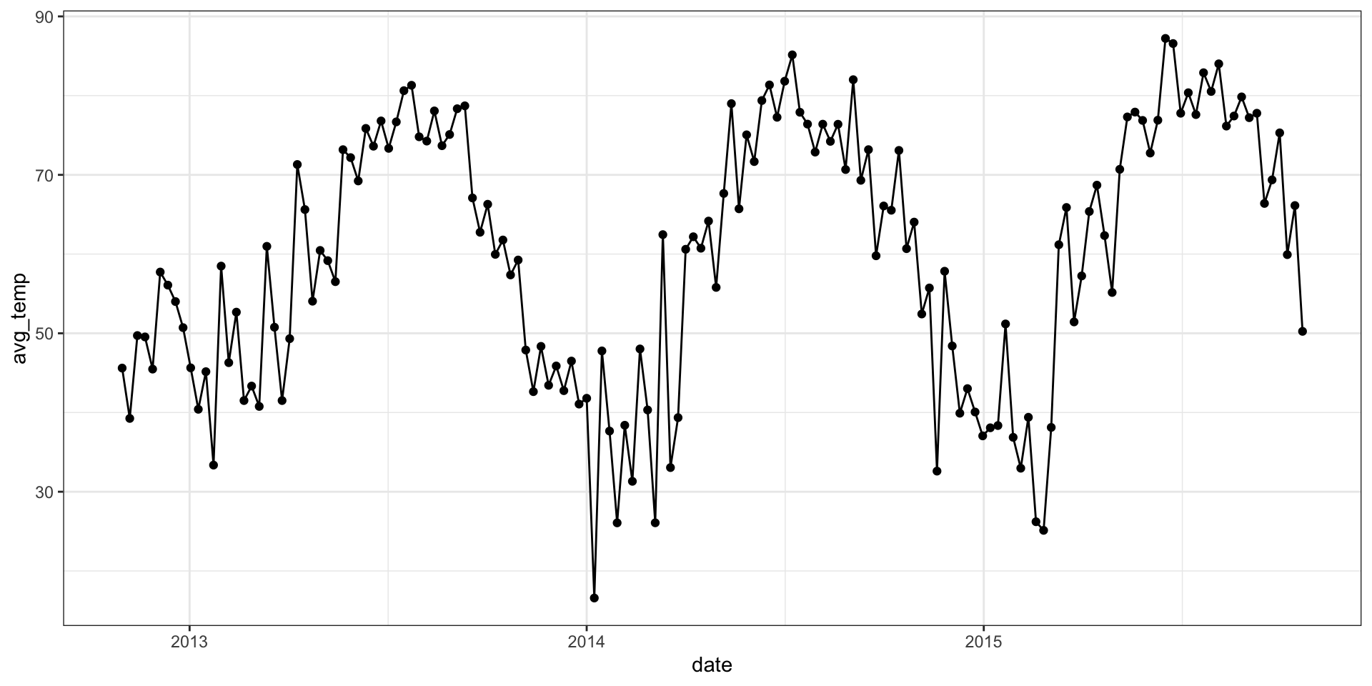
( temp = readRDS("data/avg_temp_df.rds") %>%
    slice(1:(52*3)) %>%
    mutate(week = as.numeric(date - date[1])/7) )

# A tibble: 156 × 3
   date       avg_temp  week
   <date>        <dbl> <dbl>
 1 2012-10-31     45.6     0
 2 2012-11-07     39.3     1
 3 2012-11-14     49.7     2
 4 2012-11-21     49.5     3
 5 2012-11-28     45.5     4
 6 2012-12-05     57.7     5
 7 2012-12-12     56.1     6
 8 2012-12-19     54.0     7
 9 2012-12-26     50.7     8
10 2013-01-02     45.6     9
# … with 146 more rows

ggplot(temp, aes(x=date, y=avg_temp)) +
  geom_line() +
  geom_point()

Empirical semi-variogram

emp_semivariogram(
  d=temp, y=avg_temp, x=week, 
  bin=TRUE, binwidth=c(3,5,7)
) %>% 
  ggplot(aes(x=d, y=gamma, size=n)) +
    geom_point(alpha=0.5) +
    facet_wrap(~paste0("binwidth=",bw), ncol=2) +
    ylim(0,NA)

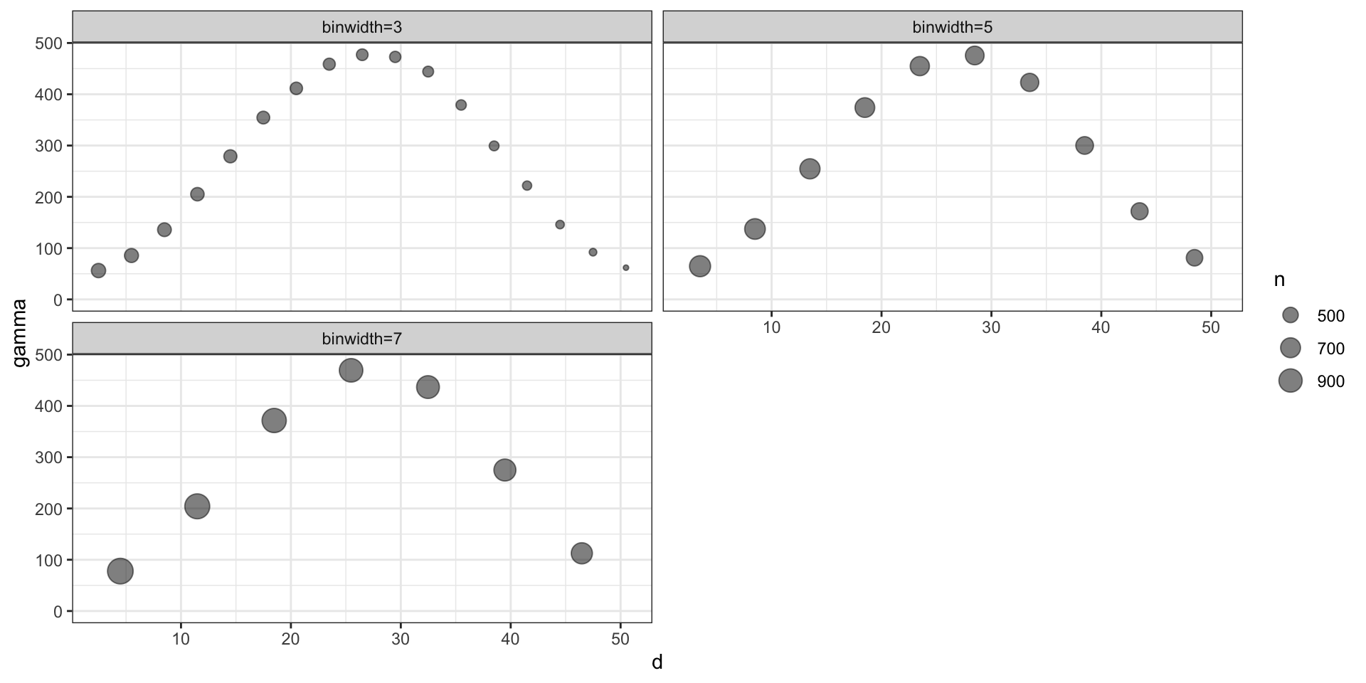
Model fitting

m = gplm(
  avg_temp~1, data = temp, coords = "week",
  cov_model = "gaussian",
  starting=list(
    "phi"=sqrt(3)/4, "sigma.sq"=1, "tau.sq"=1
  ),
  tuning=list(
    "phi"=1, "sigma.sq"=1, "tau.sq"=1
  ),
  priors=list(
    "phi.unif"=c(sqrt(3)/52, sqrt(3)/1),
    "sigma.sq.ig"=c(2, 1),
    "tau.sq.ig"=c(2, 1)
  ),
  thin = 5,
  n_batch = 100,
  batch_len = 100
)

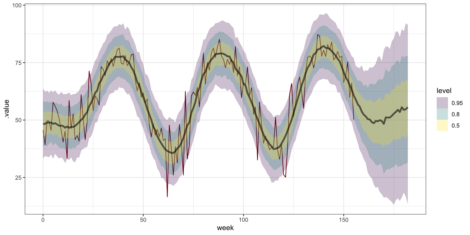
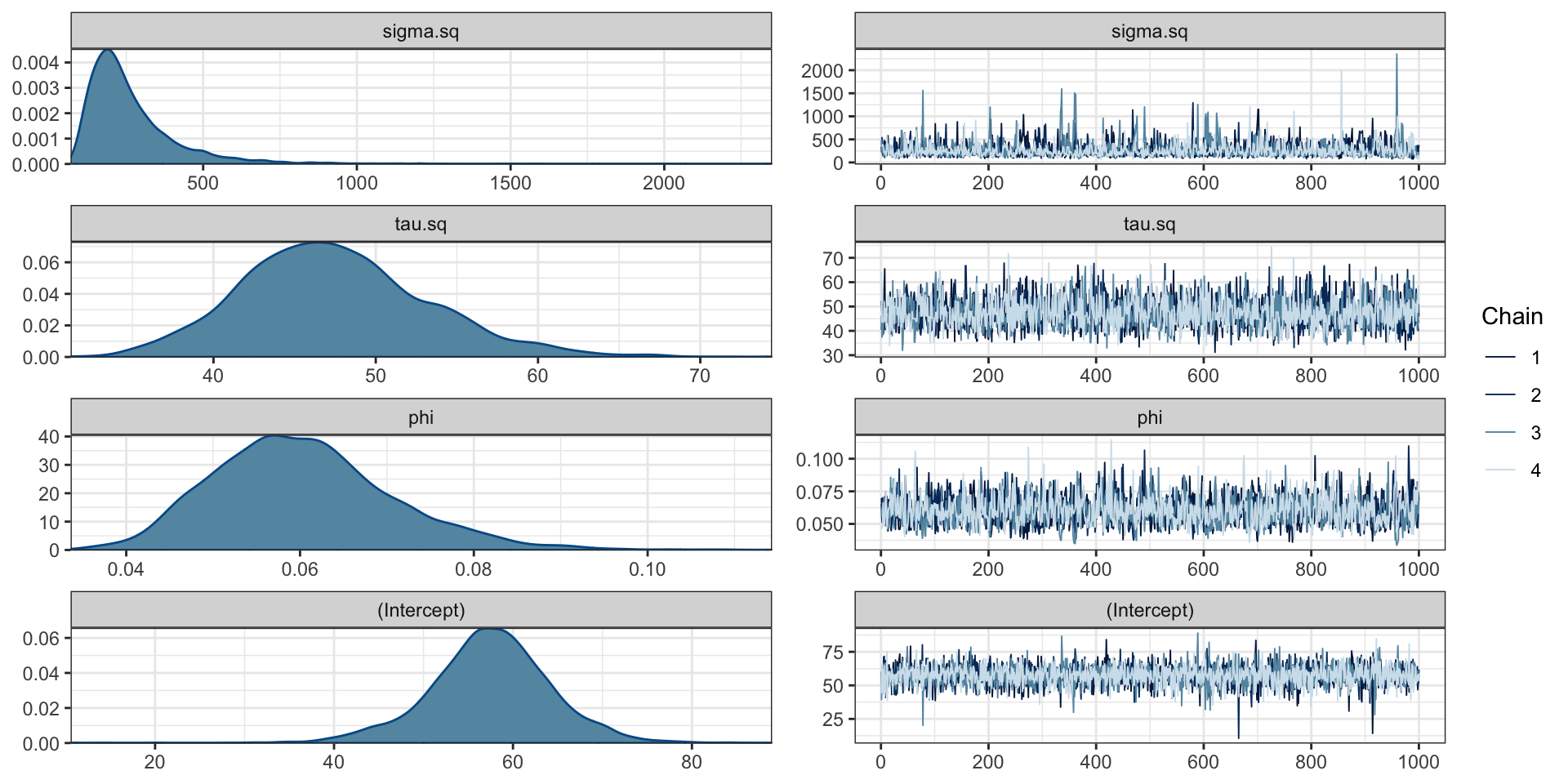
Model plots

plot(m)

Prediction

newdata = data.frame(
  week = seq(0,3.5*52) |> jitter()
)

(p = predict(m, newdata=newdata, coords = "week"))

# A draws_matrix: 1000 iterations, 4 chains, and 183 variables
    variable
draw y[1] y[2] y[3] y[4] y[5] y[6] y[7] y[8]
  1    38   45   57   42   43   47   43   55
  2    51   54   47   47   46   36   50   46
  3    42   56   45   57   36   54   48   60
  4    48   43   52   39   53   48   54   59
  5    39   38   39   46   50   50   49   48
  6    65   43   50   45   48   43   55   57
  7    43   52   56   60   54   71   40   58
  8    51   35   55   48   54   45   45   49
  9    50   48   42   44   38   52   58   40
  10   38   44   33   49   41   49   48   54
# ... with 3990 more draws, and 175 more variables

Results

p |>
  tidybayes::gather_draws(y[i]) |>
  mutate(week = i-1) |>
  filter(.chain == 1) |>
  ggplot(aes(x=week, y=.value)) +
    geom_line(data=temp, aes(y=avg_temp), color="darkred") +
    tidybayes::stat_lineribbon(alpha=0.25)

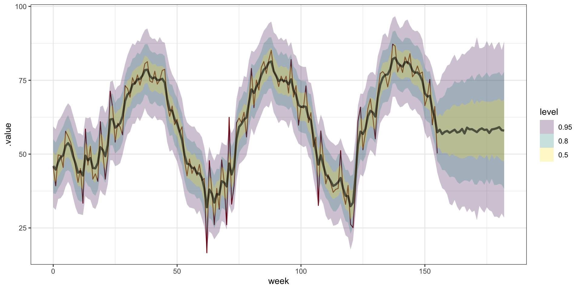
Exponential covariance

m_exp = gplm(
  avg_temp~1, data = temp, coords = "week",
  cov_model = "exponential",
  starting=list(
    "phi"=3/4, "sigma.sq"=1, "tau.sq"=1
  ),
  tuning=list(
    "phi"=1, "sigma.sq"=1, "tau.sq"=1
  ),
  priors=list(
    "phi.unif"=c(3/52, 3/1),
    "sigma.sq.ig"=c(2, 1),
    "tau.sq.ig"=c(2, 1)
  ),
  thin = 5,
  n_batch = 100,
  batch_len = 100
)

p_exp = predict(m_exp, newdata=newdata, coords = "week")

Results

p_exp |>
  tidybayes::gather_draws(y[i]) |>
  mutate(week = i-1) |>
  filter(.chain == 1) |>
  ggplot(aes(x=week, y=.value)) +
    geom_line(data=temp, aes(y=avg_temp), color="darkred") +
    tidybayes::stat_lineribbon(alpha=0.25)

More Covariance Functions

Nugget Covariance

\[ Cov(y_{t_i}, y_{t_j}) = \sigma^2 {1}_{\{h=0\}} \text{ where } h = |t_i - t_j|\]

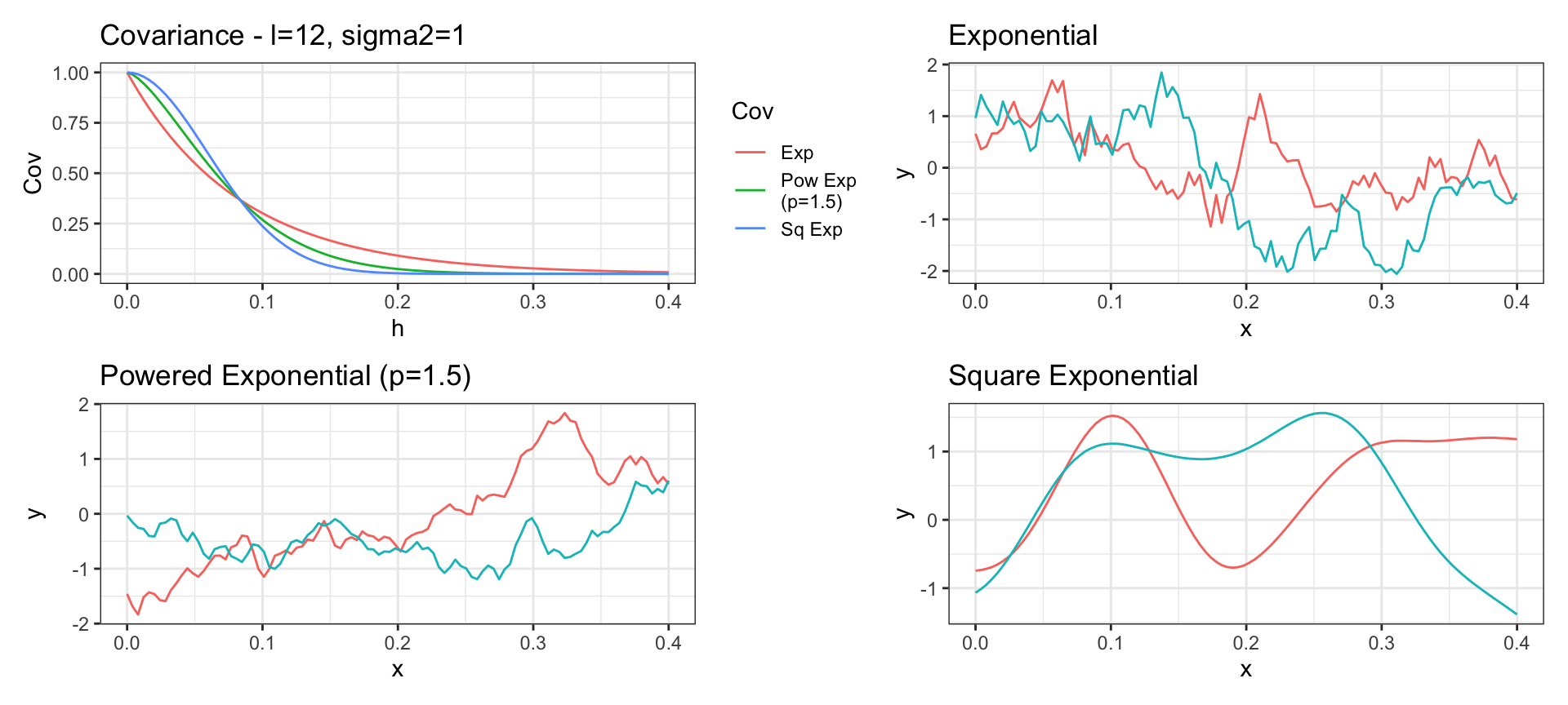
(- / Power / Square) Exponential Covariance

\[ Cov(y_{t_i}, y_{t_j}) = \sigma^2\exp\left(-(h\,l)^p\right) \text{ where } h = |t_i - t_j|\]

Matern Covariance

\[ Cov(y_{t_i}, y_{t_j}) = \sigma^2 ~ \frac{2^{1-\nu}}{\Gamma(\nu)} ~ \left(\sqrt{2\nu}\, h \cdot l\right)^\nu ~ K_\nu\left(\sqrt{2\nu} \, h \cdot l\right) \text{ where } h = |t_i - t_j|\]

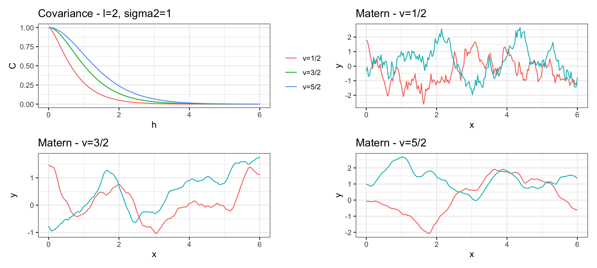
Matern Covariance

\(K_\nu()\) is the modified Bessel function of the second kind.
A Gaussian process with Matérn covariance has sample functions that are \(\lceil \nu -1\rceil\) times differentiable.
When \(\nu = 1/2 + p\) for \(p \in \mathbb{N}^+\) then the Matern has a simplified form
When \(\nu = 1/2\) the Matern is equivalent to the exponential covariance.
As \(\nu \to \infty\) the Matern converges to the squared exponential covariance.

Rational Quadratic Covariance

\[ Cov(y_{t_i}, y_{t_j}) = \sigma^2 \left(1 + \frac{h^2 \, l^2}{\alpha}\right)^{-\alpha} \text{ where } h = |t_i - t_j|\]

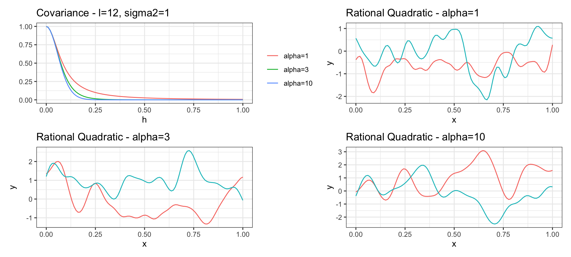
Rational Quadratic Covariance

is a scaled mixture of squared exponential covariance functions with different characteristic length-scales (\(l\)).
As \(\alpha \to \infty\) the rational quadratic converges to the square exponential covariance.
Has sample functions that are infinitely differentiable for any value of \(\alpha\)

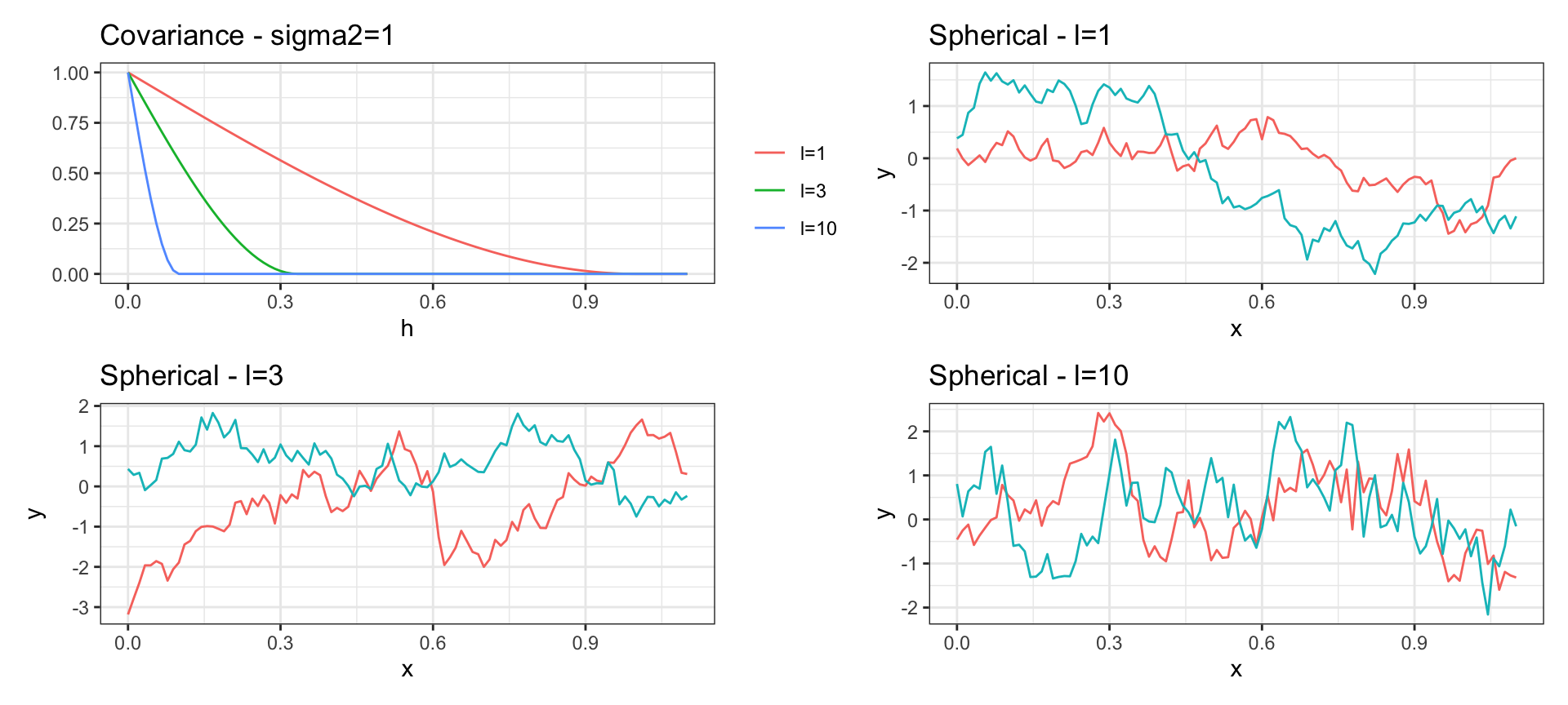
Spherical Covariance

\[ Cov(y_{t_i}, y_{t_j}) = \begin{cases} \sigma^2\left(1 - \frac{3}{2} h \cdot l + \frac{1}{2} (h \cdot l)^3)\right) & \text{if } 0 < h < 1/l \\ 0 & \text{otherwise} \end{cases} \text{ where } h = |t_i - t_j|\]

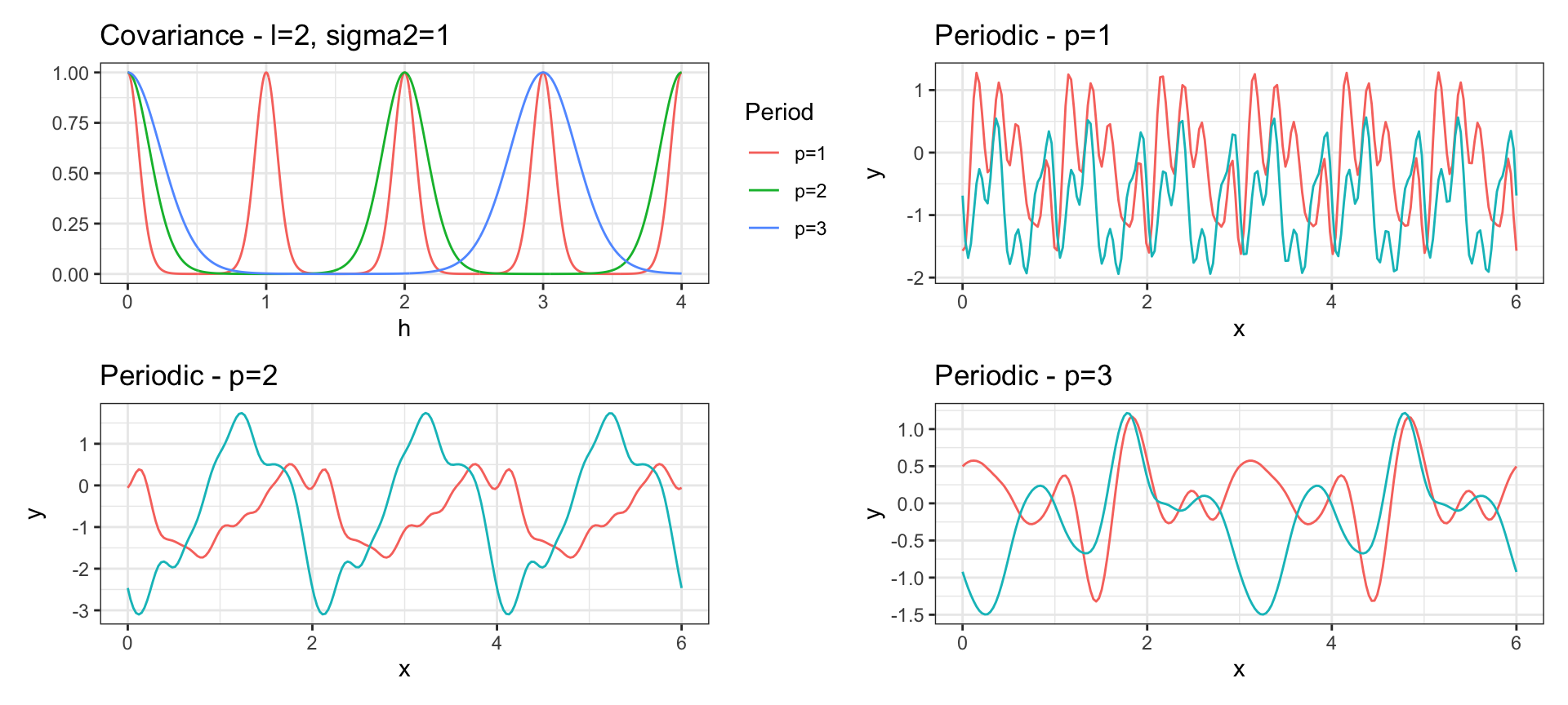
Periodic Covariance

\[ Cov(y_{t_i}, y_{t_j}) = \sigma^2 \exp\left(-2\, l^2 \sin^2\left(\pi\frac{h}{p}\right)\right) \text{ where } h = |t_i - t_j| \]

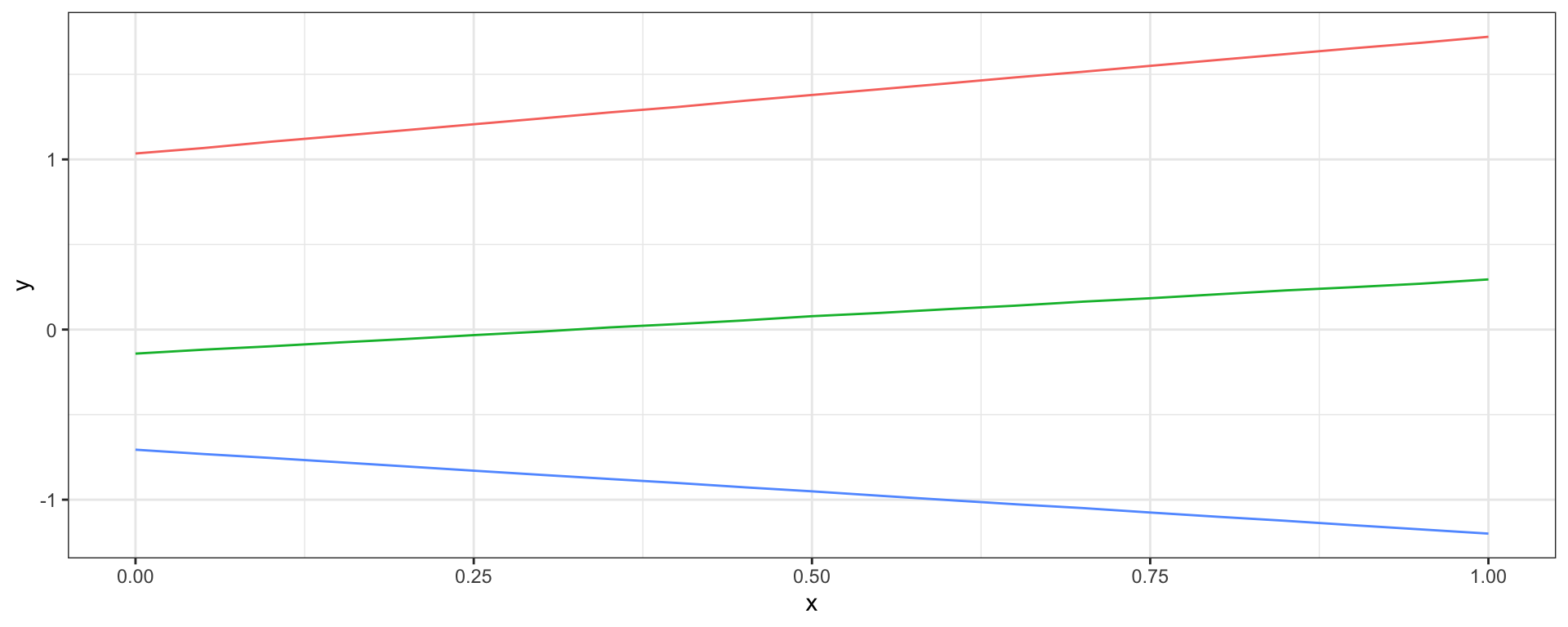
Linear Covariance

\[ Cov(y_{t_i}, y_{t_j}) = \sigma^2_b + \sigma^2_v~(t_i-c)(t_j-c)\]

Combining Covariances

If we definite two valid covariance functions, \(Cov_a(y_{t_i}, y_{t_j})\) and \(Cov_b(y_{t_i}, y_{t_j})\) then the following are also valid covariance functions,

\[ \begin{aligned} Cov_a(y_{t_i}, y_{t_j}) + Cov_b(y_{t_i}, y_{t_j}) \\ \\ Cov_a(y_{t_i}, y_{t_j}) \times Cov_b(y_{t_i}, y_{t_j}) \end{aligned} \]

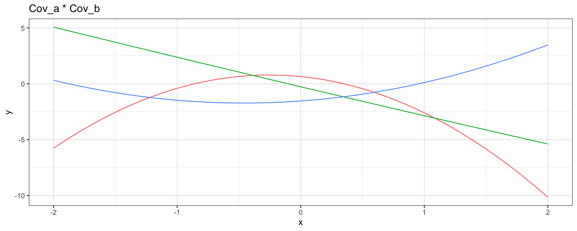
Linear \(\times\) Linear \(\to\) Quadratic

\[ Cov_a(y_{t_i}, y_{t_j}) = 1 + 2~(t_i \times t_j) \] \[ Cov_b(y_{t_i}, y_{t_j}) = 2 + 1~(t_i \times t_j) \]

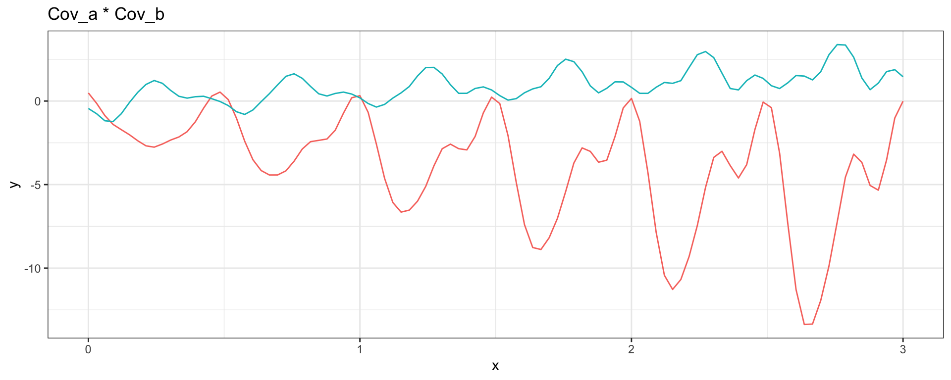
Linear \(\times\) Periodic

\[ Cov_a(y_{t_i}, y_{t_j}) = 1 + 1~(t_i \times t_j) \] \[ Cov_b(y_{t_i}, y_{t_j}) = \exp\left(-2\, \sin^2\left(2\pi\,h\right)\right) \]

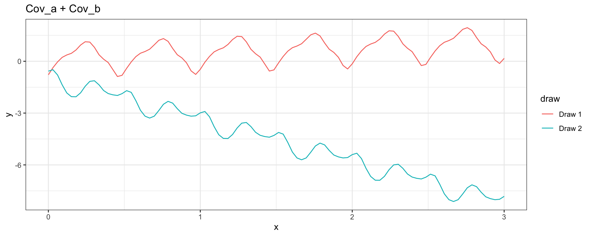
Linear + Periodic

\[ Cov_a(y_{t_i}, y_{t_j}) = 1 + 1~(t_i \times t_j) \] \[ Cov_b(h = |t_i - t_j|) = \exp\left(-2\, \sin^2\left(2\pi\,h\right)\right) \]

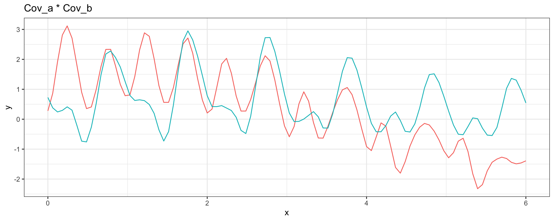
Sq Exp \(\times\) Periodic \(\to\) Locally Periodic

\[ Cov_a(h = |t_i - t_j|) =\exp(-(1/3)h^2) \] \[ Cov_b(h = |t_i - t_j|) = \exp\left(-2\, \sin^2\left(\pi\,h\right)\right) \]

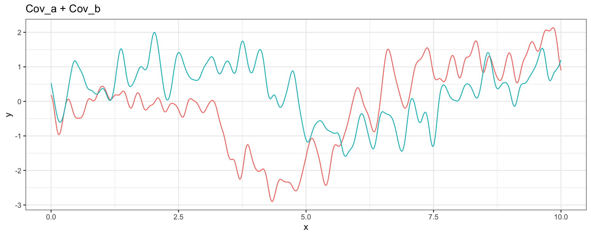
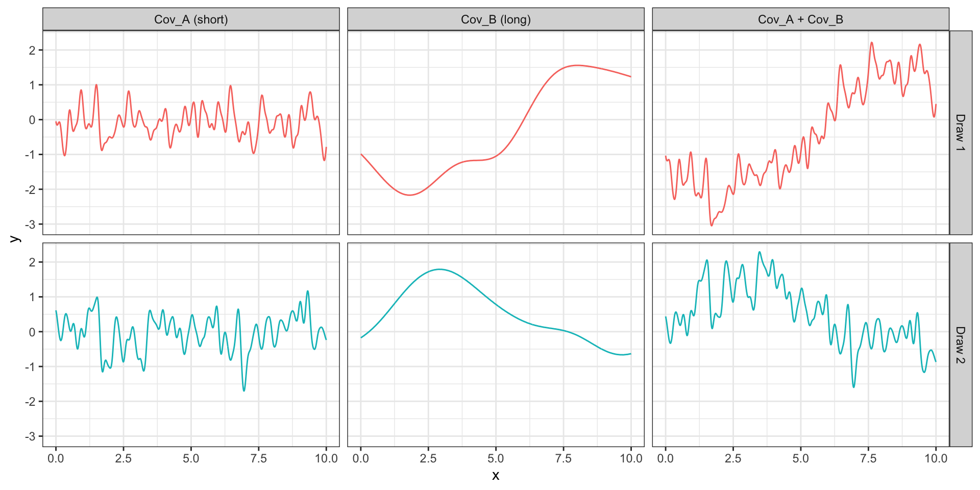
Sq Exp (short) + Sq Exp (long)

\[ Cov_a(h = |t_i - t_j|) = (1/4) \exp(-4\sqrt{3}h^2) \] \[ Cov_b(h = |t_i - t_j|) = \exp(-(\sqrt{3}/2)h^2) \]

Seen another way

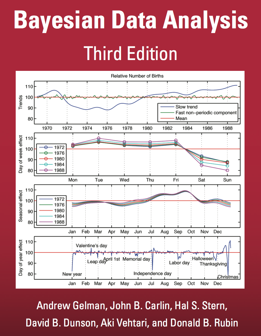
BDA3 example

BDA3

Births (one year)

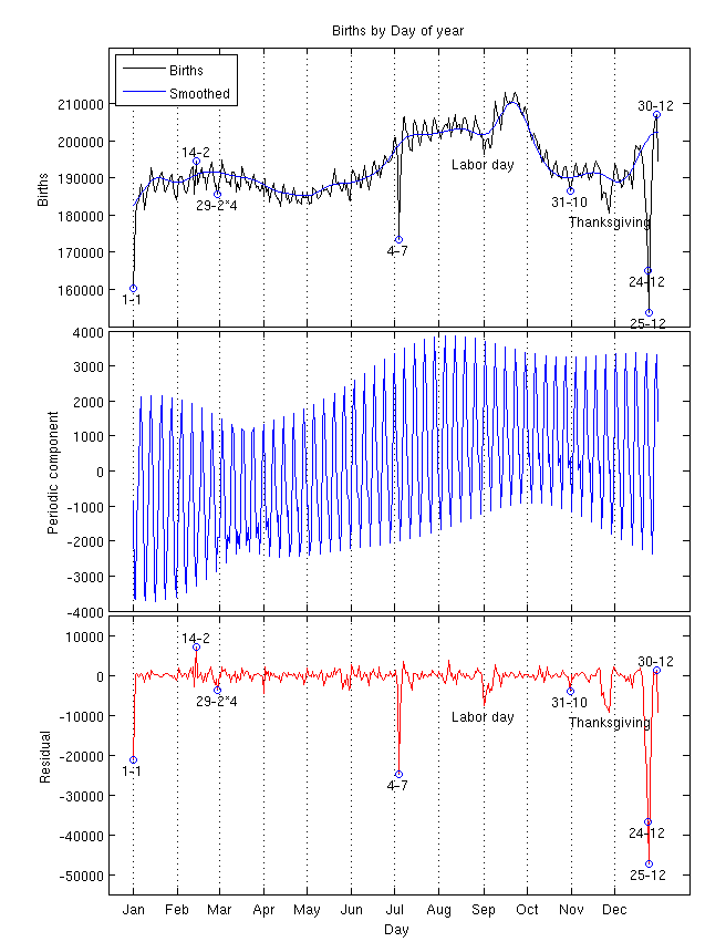
Smooth long term trend
(sq exp cov)
Seven day periodic trend with decay (periodic x sq exp cov)
Constant mean

Component Contributions

We can view our GP in the following ways (marginal form),

\[ \boldsymbol{y} \sim N(\boldsymbol{\mu},~ \boldsymbol{\Sigma}_1 + \boldsymbol{\Sigma}_2 + \sigma^2 \boldsymbol{I}\,) \]

but with appropriate conditioning we can also think of \(\boldsymbol{y}\) as being the sum of multiple independent GPs (latent form)

\[ \boldsymbol{y} = \boldsymbol{\mu} + w_1(\boldsymbol{t}) + w_2(\boldsymbol{t}) + w_3(\boldsymbol{t})\] where \[ \begin{aligned} w_1(\boldsymbol{t}) &\sim N(0, \boldsymbol{\Sigma}_1) \\ w_2(\boldsymbol{t}) &\sim N(0, \boldsymbol{\Sigma}_2) \\ w_3(\boldsymbol{t}) &\sim N(0, \sigma^2 \boldsymbol{I}\,) \end{aligned} \]

Decomposition of Covariance Components

\[ \begin{bmatrix} y \\ w_1 \\ w_2 \end{bmatrix} \sim N \left( \begin{bmatrix} \boldsymbol{\mu} \\ 0 \\ 0 \end{bmatrix},~ \begin{bmatrix} \Sigma_1 + \Sigma_2 + \sigma^2 \boldsymbol{I} & \Sigma_1 & \Sigma_2 \\ \Sigma_1 & \Sigma_1 & 0\\ \Sigma_2 & 0 & \Sigma_2 \\ \end{bmatrix} \right) \]

therefore

\[ w_1 ~|~ \boldsymbol{y},\boldsymbol{\mu},\boldsymbol{\theta} \sim N(\boldsymbol{\mu}_{cond},~ \boldsymbol{\Sigma}_{cond}) \]

\[ \boldsymbol{\mu}_{cond} = 0 + \Sigma_1 ~ (\Sigma_1 + \Sigma_2 + \sigma^2 I)^{-1}(\boldsymbol{y}-\boldsymbol{\mu}) \] \[ \boldsymbol{\Sigma}_{cond} = \Sigma_1 - \Sigma_1 (\Sigma_1 + \Sigma_2 + \sigma^2 \boldsymbol{I})^{-1} {\Sigma_1}^t \]

Births (multiple years)

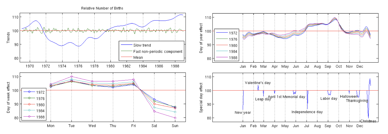
Full stan case study here with code here

slowly changing trend - yearly (sq exp cov)
small time scale trend - monthly (sq exp cov)
7 day periodic - day of week effect (periodic \(\times\) sq exp cov)
365.25 day periodic - day of year effect (periodic \(\times\) sq exp cov)
special days and interaction with weekends (linear cov)
independent Gaussian noise (nugget cov)
constant mean

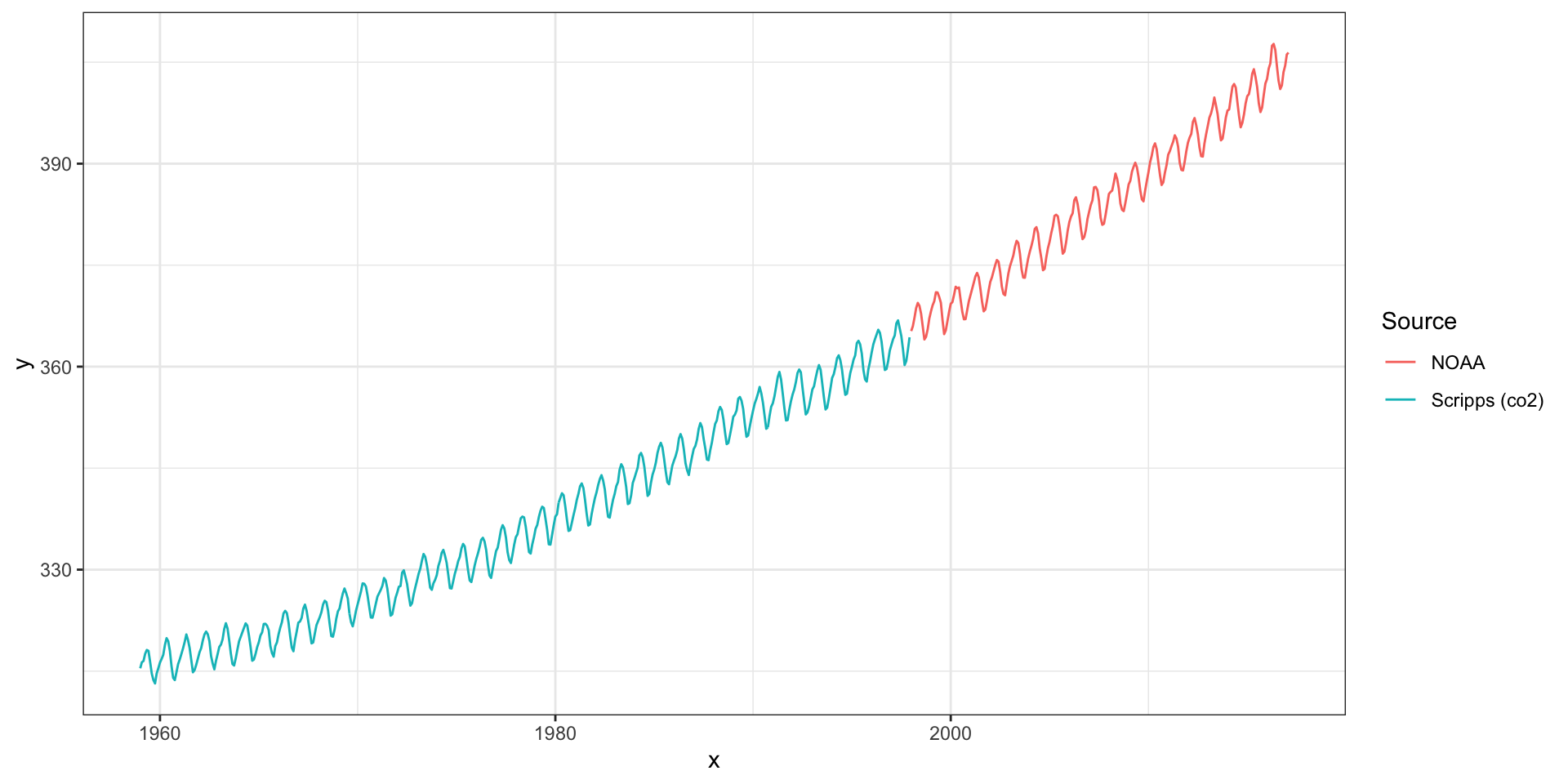
Mauna Loa Example

Atmospheric CO\(_2\)

GP Model

Based on Rasmussen 5.4.3 (we are using slightly different data and parameterization)

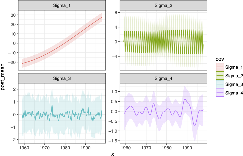
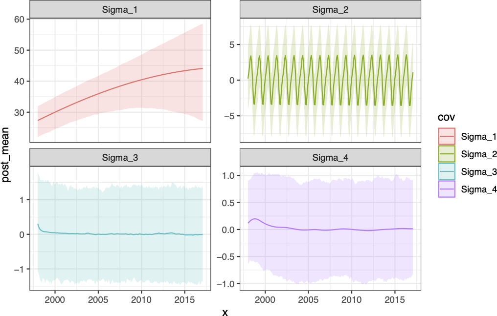
\[ \boldsymbol{y} \sim \mathcal{N}(\boldsymbol{\mu},~ \boldsymbol{\Sigma}_1 + \boldsymbol{\Sigma}_2 + \boldsymbol{\Sigma}_3 + \boldsymbol{\Sigma}_4 + \sigma^2 \mathit{I}\,) \]

\[\{\boldsymbol{\mu}\}_i = \bar{y}\]

\[ \begin{aligned} \{\boldsymbol{\Sigma}_1\}_{ij} &= \sigma^2_1 \exp\left(-(l_1 \cdot d_{ij})^2\right) \\ \{\boldsymbol{\Sigma}_2\}_{ij} &= \sigma^2_2 \exp\left(-(l_2 \cdot d_{ij})^2\right)\exp\left(-2 \, (l_3)^2 \sin^2(\pi \, d_{ij} / p)\right) \\ \{\boldsymbol{\Sigma}_3\}_{ij} &= \sigma^2_3 \left(1+\frac{(l_4 \cdot d_{ij})^2}{\alpha}\right)^{-\alpha} \\ \{\boldsymbol{\Sigma}_4\}_{ij} &= \sigma^2_4 \exp\left(-(l_5 \cdot d_{ij})^2\right) \end{aligned} \]

Model fit

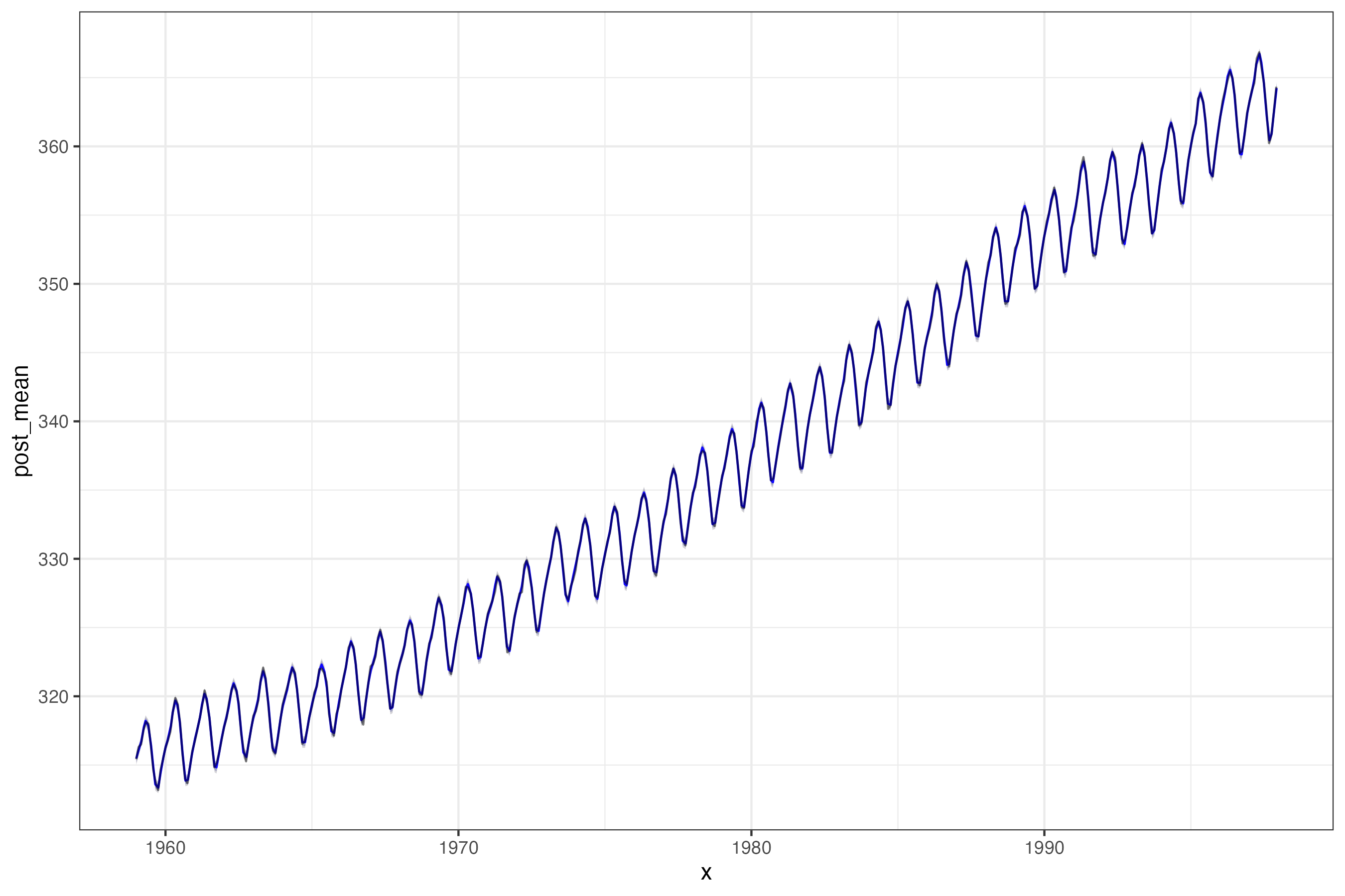
Fit Components

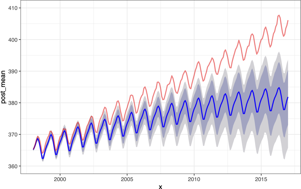
Model fit + forecast

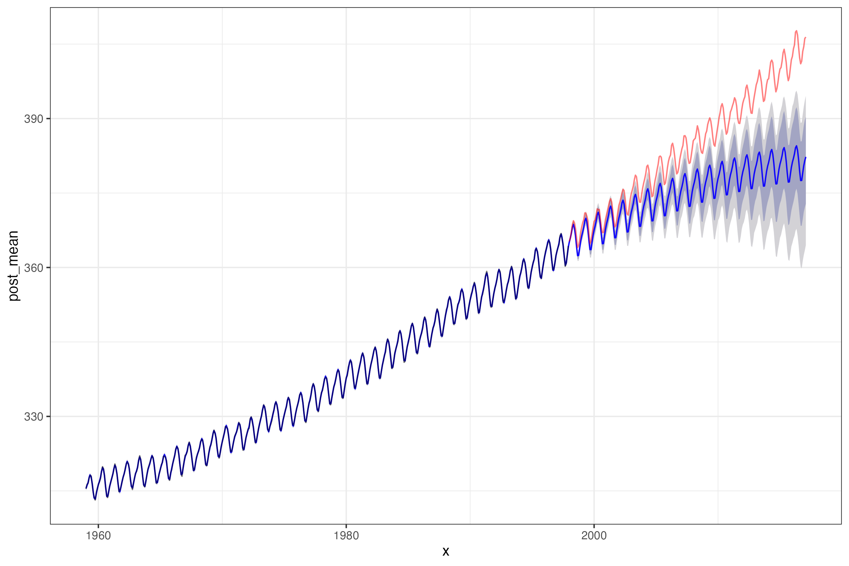
Forecast

Forecast components

ARIMA forecast

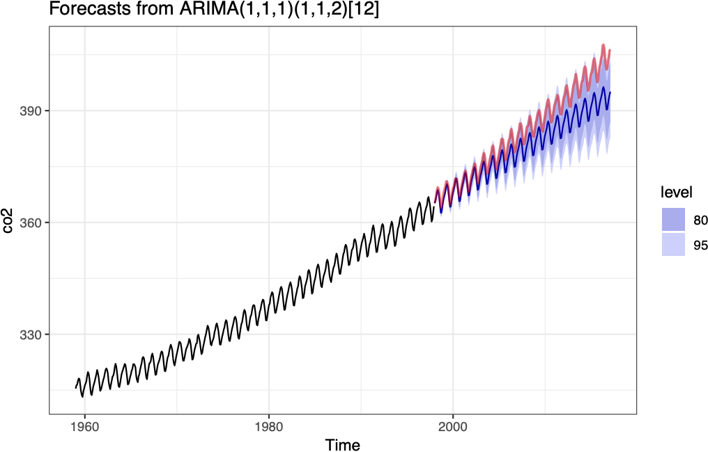
Model performance

Forecast dates	arima RMSE	gp RMSE
Jan 1998 - Jan 2003	1.10	1.91
Jan 1998 - Jan 2008	2.51	4.58
Jan 1998 - Jan 2013	3.82	7.71
Jan 1998 - Mar 2017	5.46	11.40