Gaussian Process Models
Part 2
Lecture 15
EDA and GPs
Variogram
When fitting a Gaussian process model, it is often difficult to fit the covariance parameters (hard to identify). Today we will discuss some EDA approaches for getting a sense of the values for the scale, range and nugget parameters.
From the spatial modeling literature the typical approach is to examine an empirical variogram, first we will define the theoretical variogram and its connection to the covariance.
Variogram: \[ 2 \gamma(t_i, t_j) = Var(y(t_i) - y(t_j)) \] where \(\gamma(t_i, t_j)\) is known as the semivariogram.
Properties of the Variogram / Semivariogram
- are non-negative - \(\gamma(t_i, t_j) \geq 0\)
- are equal to 0 at distance 0 - \(\gamma(t_i, t_i) = 0\)
- are symmetric - \(\gamma(t_i, t_j) = \gamma(t_j, t_i)\)
- if observations are independent \(2\gamma(t_i, t_j) = Var(y(t_i)) + Var(y(t_j)) \quad \text{ for all } i \ne j\)
- if the process is not stationary \(2\gamma(t_i, t_j) = Var\big(y(t_i)\big) + Var\big(y(t_j)\big) - 2 \, Cov\big(y(t_i),y(t_j)\big)\)
- if the process is stationary \(2\,\gamma(t_i, t_j) = 2 \, Var\big(y(t_i)\big) - 2 \, Cov\big(y(t_i),y(t_j)\big)\)
Connection to Covariance
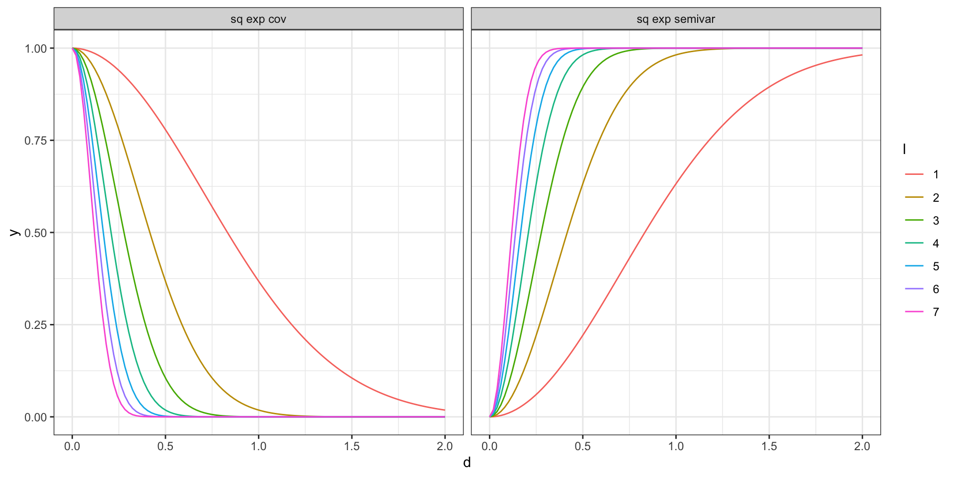
Assuming a squared exponential covariance structure,
\[ \begin{aligned} 2\gamma(t_i, t_j) &= 2Var\big(y(t_i)\big) - 2 \, Cov\big(y(t_i),y(t_j)\big) \\ \gamma(t_i, t_j) &= Var\big(y(t_i)\big) - \, Cov\big(y(t_i),y(t_j)\big) \\ &= \sigma^2 - \, \sigma^2 \exp\big(-(|t_i-t_j|\,l)^2\big) \end{aligned} \]
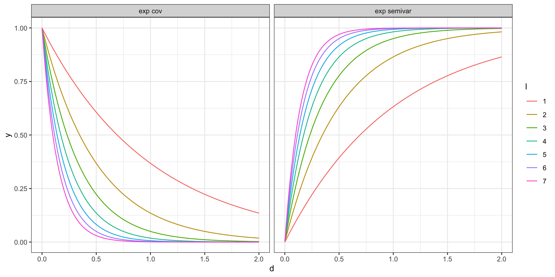
Covariance vs Semivariogram - Exponential
Covariance vs Semivariogram - Sq. Exp.
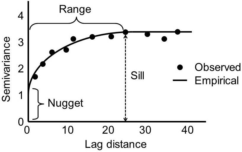
Nugget variance
Very often in the real world we will observe that \(\gamma(t_i, t_i) = 0\) is not true - there will be an initial discontinuity in the semivariogram at \(|t_i - t_j| = 0\).
Why is this?
We can think about Gaussian process regression in the following way,
\[ y(t) = \mu(t) + w(t) + \epsilon(t) \]
where
\[ \begin{aligned} \boldsymbol{\mu}(\boldsymbol{t}) &= \boldsymbol{X} \boldsymbol{\beta} \\ \boldsymbol{w}(\boldsymbol{t}) &\sim N(\boldsymbol{0}, \boldsymbol{\Sigma}) \\ \epsilon(t) &\overset{iid}{\sim} N(0, \sigma^2_w)\\ \end{aligned} \]
Implications
With the inclusion of the \(\epsilon(t)\) terms in the model we now have,
\[ \begin{aligned} Var\big(y(t_i)\big) &= \sigma^2_w + \Sigma_{ii} \\ Cov\big(y(t_i), y(t_j)\big) &= \Sigma_{ij} \end{aligned} \]
Therefore, for a squared exponential covariance model with a nugget component the semivariogram is given by,
\[ \gamma(t_i,t_j) = \left(\sigma^2 + \sigma^2_w \right) - \sigma^2 \exp \left(- (|t_i-t_j|\,l)^2\right) \]
Semivariogram features
Empirical Semivariogram
We will assume that our process of interest is stationary, in which case we will parameterize the semivariagram in terms of \(d = |t_i - t_j|\).
Empirical Semivariogram: \[ \hat{\gamma}(d) = \frac{1}{2 \, N(d)} \sum_{|t_i-t_j| \in (d-\epsilon,d+\epsilon)} (y(t_i) - y(t_j))^2 \]
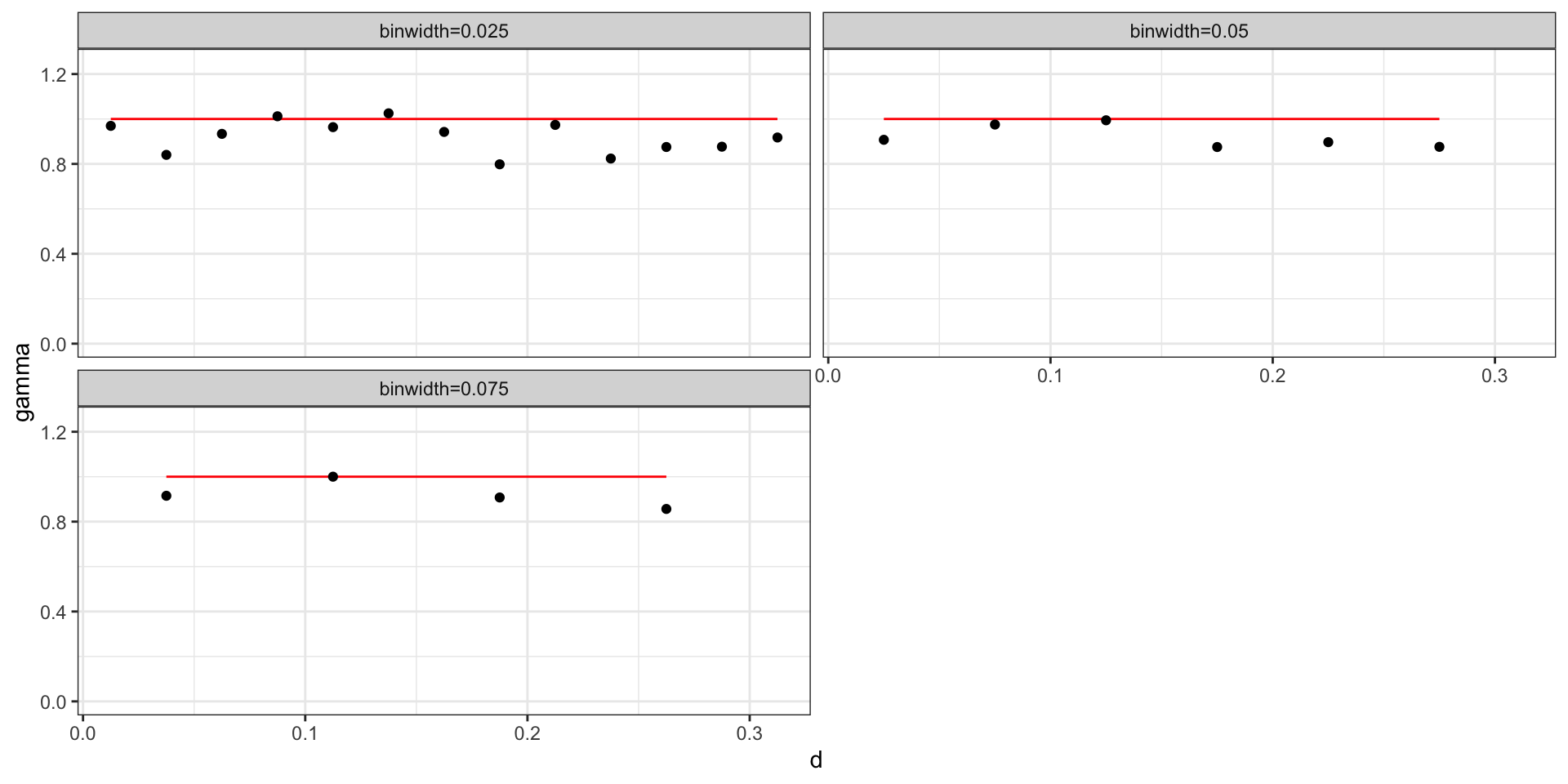
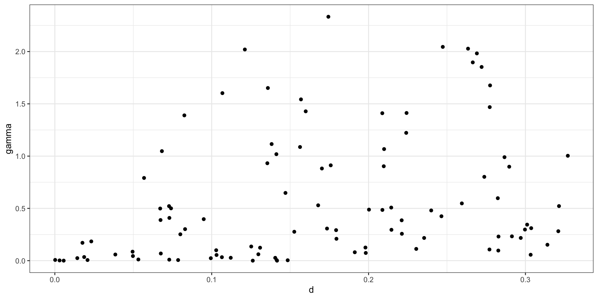
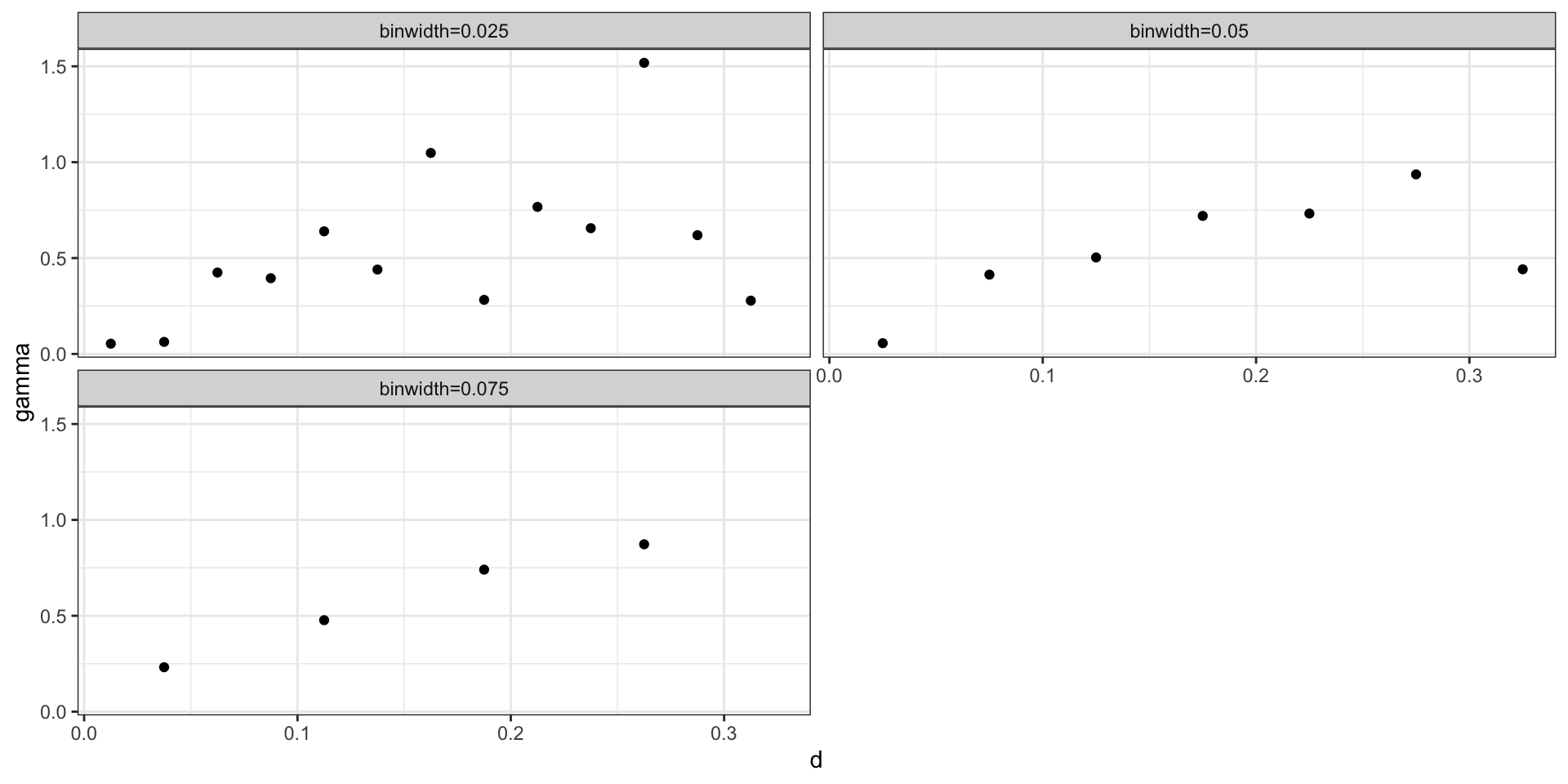
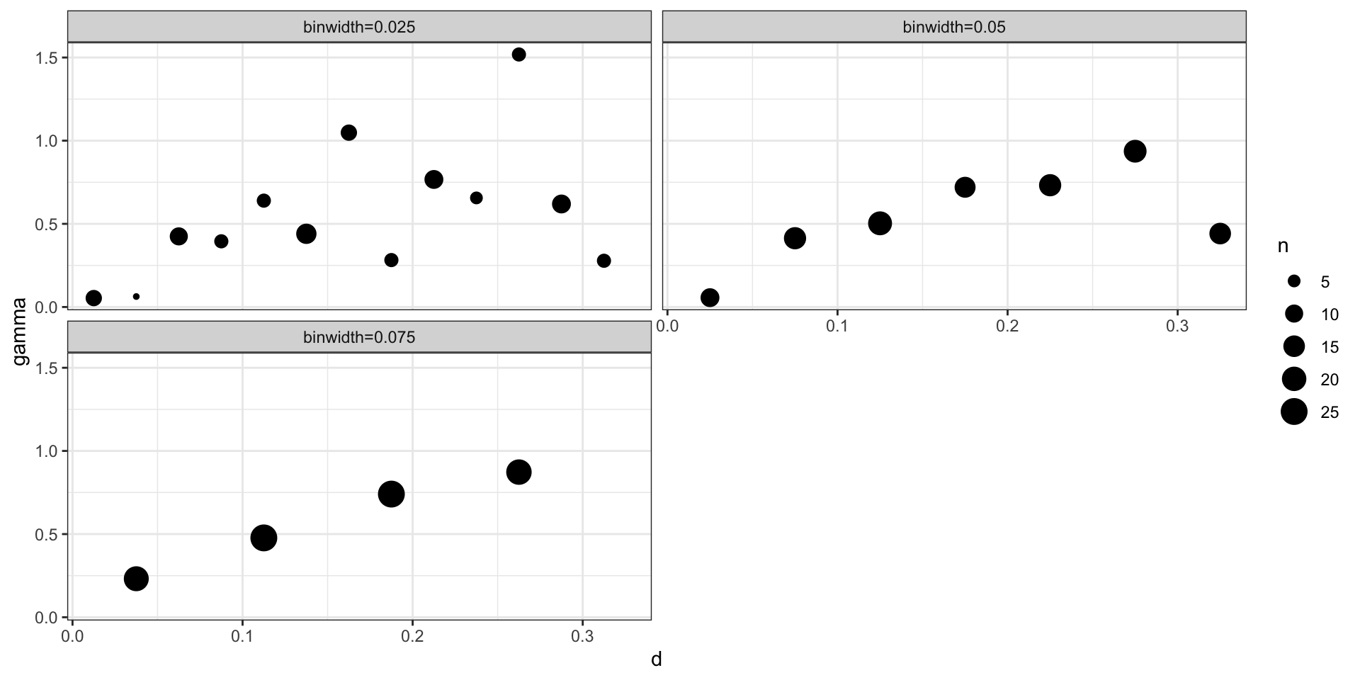
Practically, for any data set with \(n\) observations there are \({n \choose 2} + n\) possible data pairs to examine. Each individually is not very informative, so we aggregate into bins and calculate the empirical semivariogram for each bin.
Empirical semivariogram of WN
Where \(\sigma^2_w = 1\),
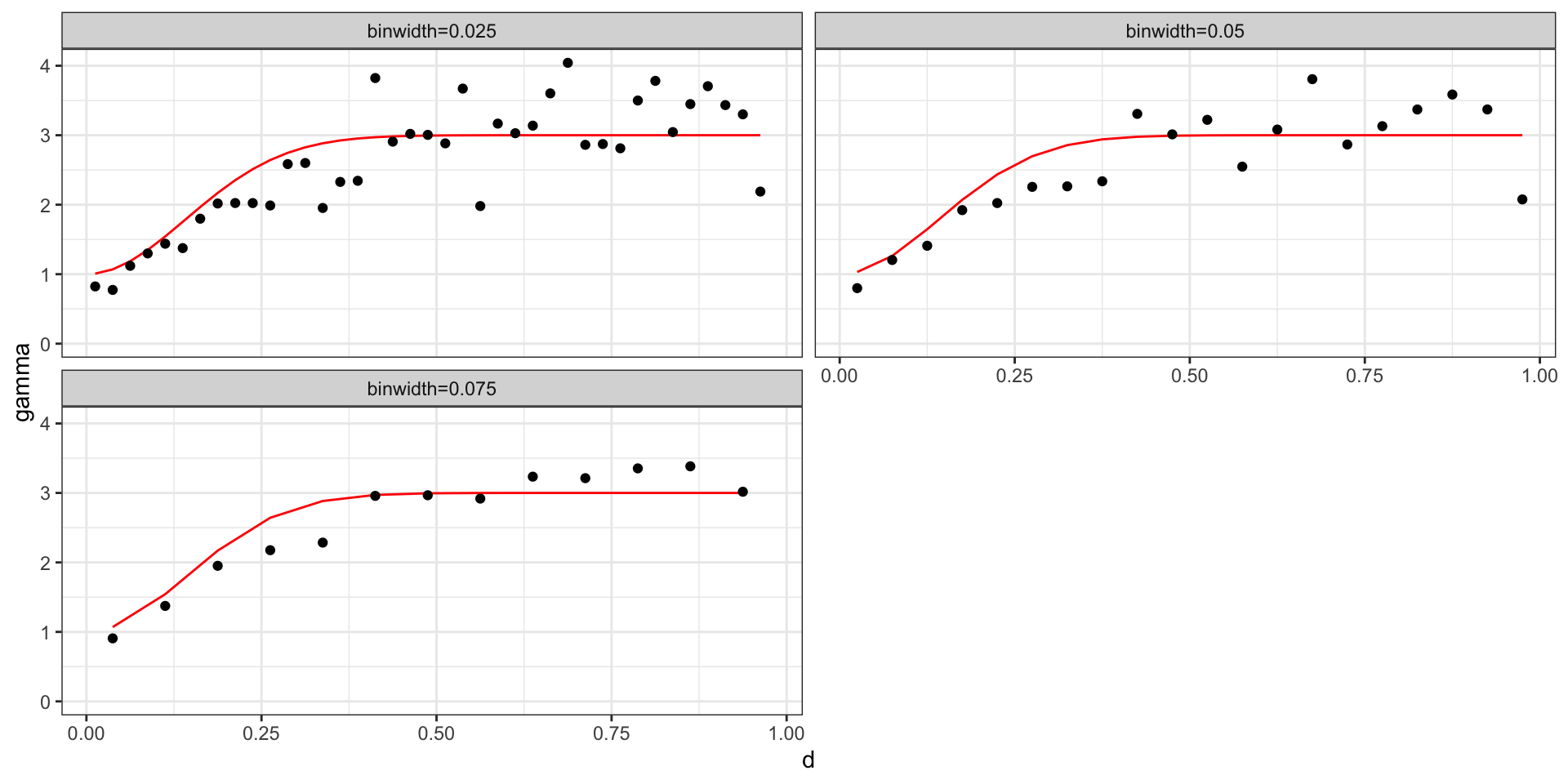
Empirical Variogram of GP w/ Sq Exp
Where \(\sigma^2=2\), \(l=5\), and \(\sigma^2_w=1\),
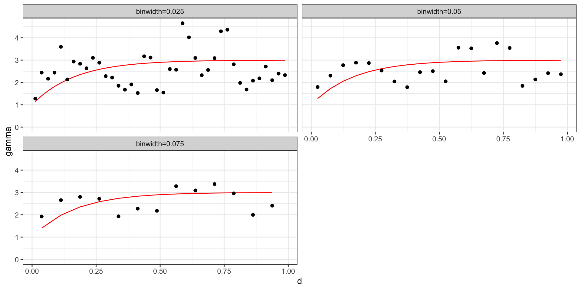
Empirical Variogram of GP w/ Exp
Where \(\sigma^2=2\), \(l=6\), and \(\sigma^2_w=1\),
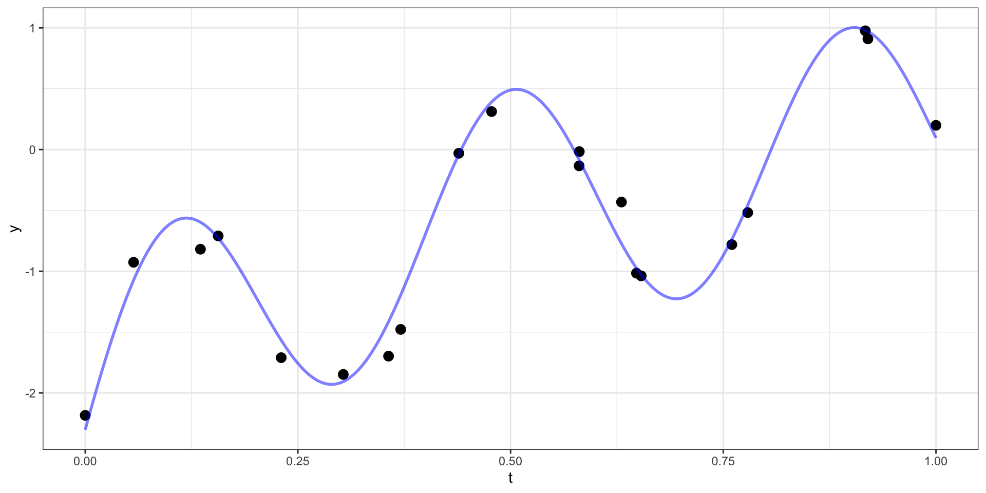
From last time
Empirical semivariogram - no bins / cloud
Empirical semivariogram (binned)
Empirical semivariogram (binned w/ size)
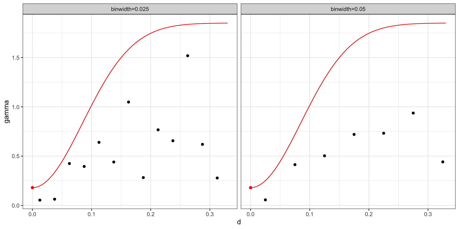
Theoretical vs empirical semivariogram
After fitting the model last time we came up with a posterior mean of \(\sigma^2 = 1.67\), \(l=8.33\), and \(\sigma^2_w\) = 0.18 for a square exponential covariance.
\[ \begin{aligned} Cov(d) &= \sigma^2 \exp\big(-(d\,l)^2\big) + \sigma^2_w \boldsymbol{1}_{h=0}\\ \gamma(h) &= (\sigma^2 + \sigma^2_w) - \sigma^2 \exp\big(-(h\,l)^2\big) \\ &= (1.67 + 0.18) - 1.67 \exp\big(-(8.33\, h)^2\big) \end{aligned} \]
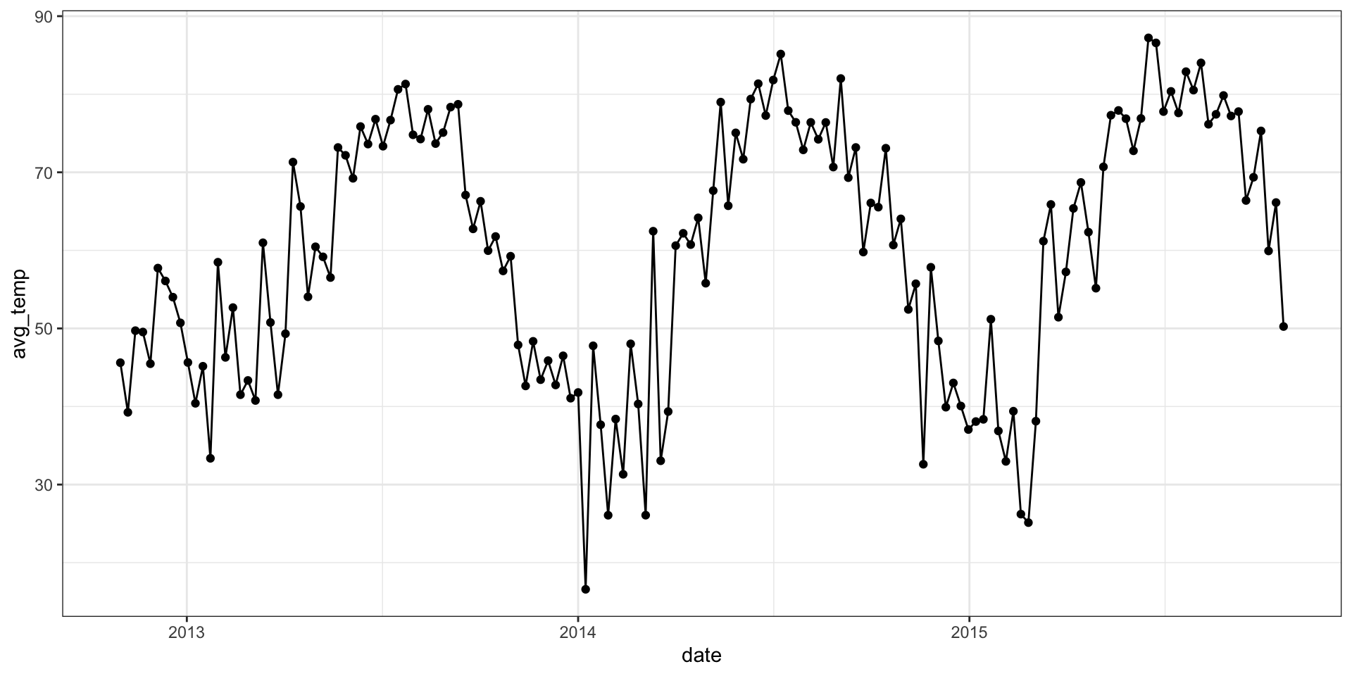
Durham Average Daily Temperature
Temp Data
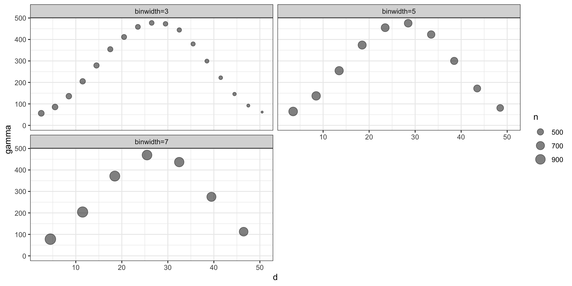
Empirical semivariogram
Model
What does the model we are trying to fit actually look like?
\[ y(t) = \mu(t) + w(t) + \epsilon(t) \]
where
\[ \begin{aligned} \boldsymbol{\mu(t)} &= \beta_0 \\ \boldsymbol{w(t)} &\sim \mathcal{GP}(0, \boldsymbol{\Sigma}) \\ \epsilon(t) &\sim \mathcal{N}(0, \sigma^2_w)\\ \\ \{\boldsymbol{\Sigma}\}_{ij} &= Cov(t_i, t_j) = \sigma^2 \exp(- (|t_i-t_j|\,l)^2) \end{aligned} \]
BRMS Model
 Family: gaussian
  Links: mu = identity; sigma = identity
Formula: avg_temp ~ 1 + gp(week)
   Data: temp (Number of observations: 156)
  Draws: 4 chains, each with iter = 2000; warmup = 1000; thin = 1;
         total post-warmup draws = 4000

Gaussian Process Terms:
               Estimate Est.Error l-95% CI u-95% CI Rhat Bulk_ESS Tail_ESS
sdgp(gpweek)      14.41      6.80     2.56    19.33 4.69        4       12
lscale(gpweek)     0.22      0.10     0.05     0.33 3.44        4       12

Population-Level Effects:
          Estimate Est.Error l-95% CI u-95% CI Rhat Bulk_ESS Tail_ESS
Intercept     2.42      2.28    -0.63     5.15 4.66        4       NA

Family Specific Parameters:
      Estimate Est.Error l-95% CI u-95% CI Rhat Bulk_ESS Tail_ESS
sigma    40.10     15.75    17.18    61.32 5.03        4        9

Draws were sampled using sampling(NUTS). For each parameter, Bulk_ESS
and Tail_ESS are effective sample size measures, and Rhat is the potential
scale reduction factor on split chains (at convergence, Rhat = 1).
BRMS Alternatives
The BRMS model (and hence Stan) took >10 minutes (per chain) to attempt to fit the model and failed spectacularly.
We could improve things slightly by tweaking the priors and increasing iterations but this wont solve the slowness issue.
The stop gap work around - using spBayes
Interface is old and clunky (inputs and outputs)
Designed for spatial GPs
Super fast (~10 seconds for 20k iterations)
I am working on a wrapper to make the interface / usage not as terrible (more next week)
Fitting a model
# A gplm model (spBayes spLM) with 4 chains, 4 variables, and 4000 iterations.
# A tibble: 4 × 10
variable mean median sd mad q5 q95 rhat ess_b…¹ ess_t…²
<chr> <dbl> <dbl> <dbl> <dbl> <dbl> <dbl> <dbl> <dbl> <dbl>
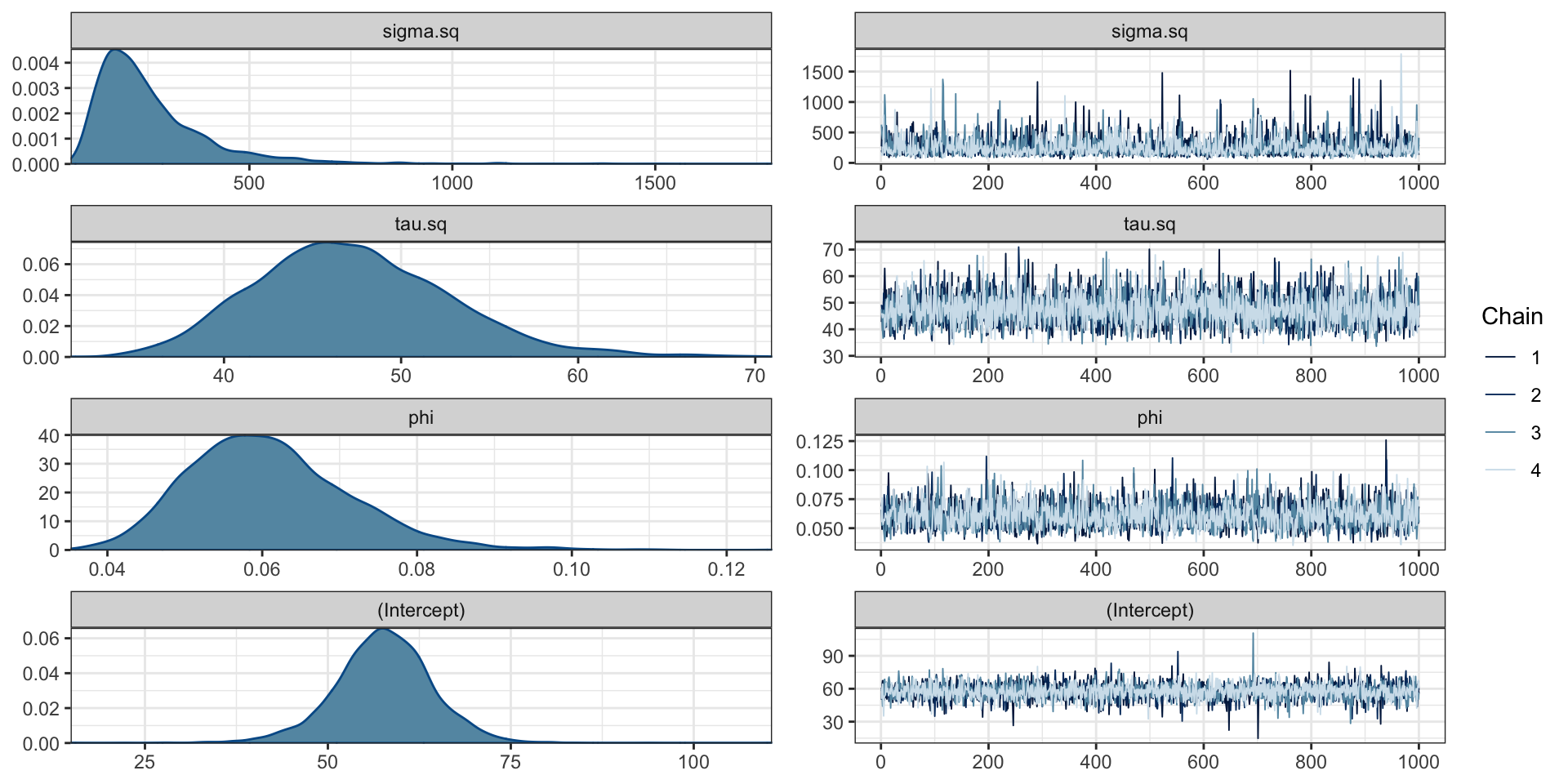
1 sigma.sq 2.58e+2 2.18e+2 1.50e+2 9.85e+1 1.11e+2 5.34e+2 1.00 2837. 3108.
2 tau.sq 4.73e+1 4.69e+1 5.56e+0 5.42e+0 3.89e+1 5.68e+1 0.999 4055. 3893.
3 phi 6.09e-2 6.00e-2 1.05e-2 9.89e-3 4.58e-2 7.91e-2 1.00 2988. 3158.
4 (Interc… 5.76e+1 5.77e+1 6.75e+0 6.12e+0 4.64e+1 6.83e+1 1.00 4081. 3535.
# … with abbreviated variable names ¹ess_bulk, ²ess_tailParameter posteriors
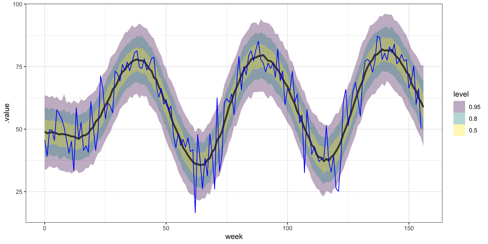
Fitted model
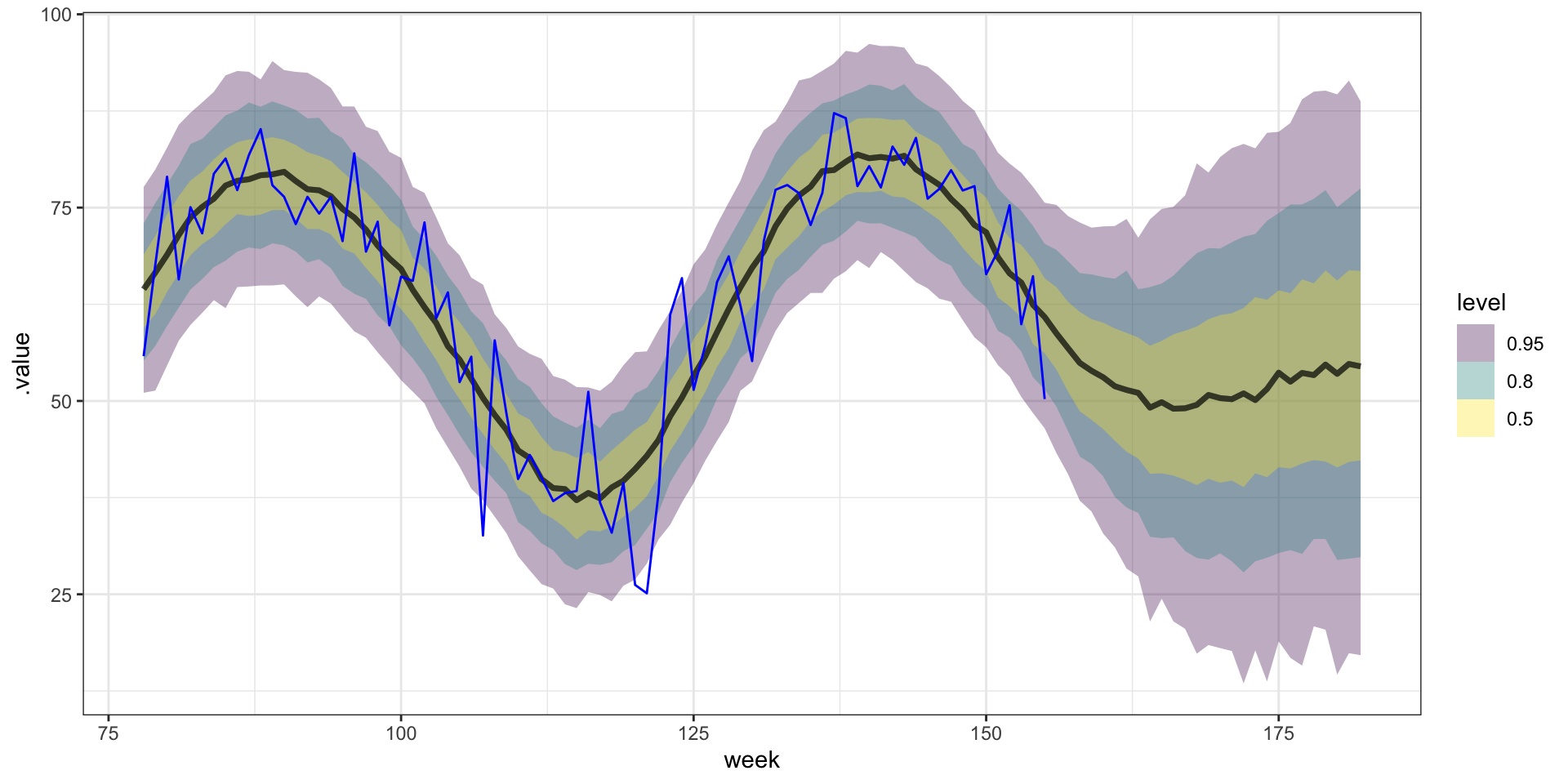
Forecasting
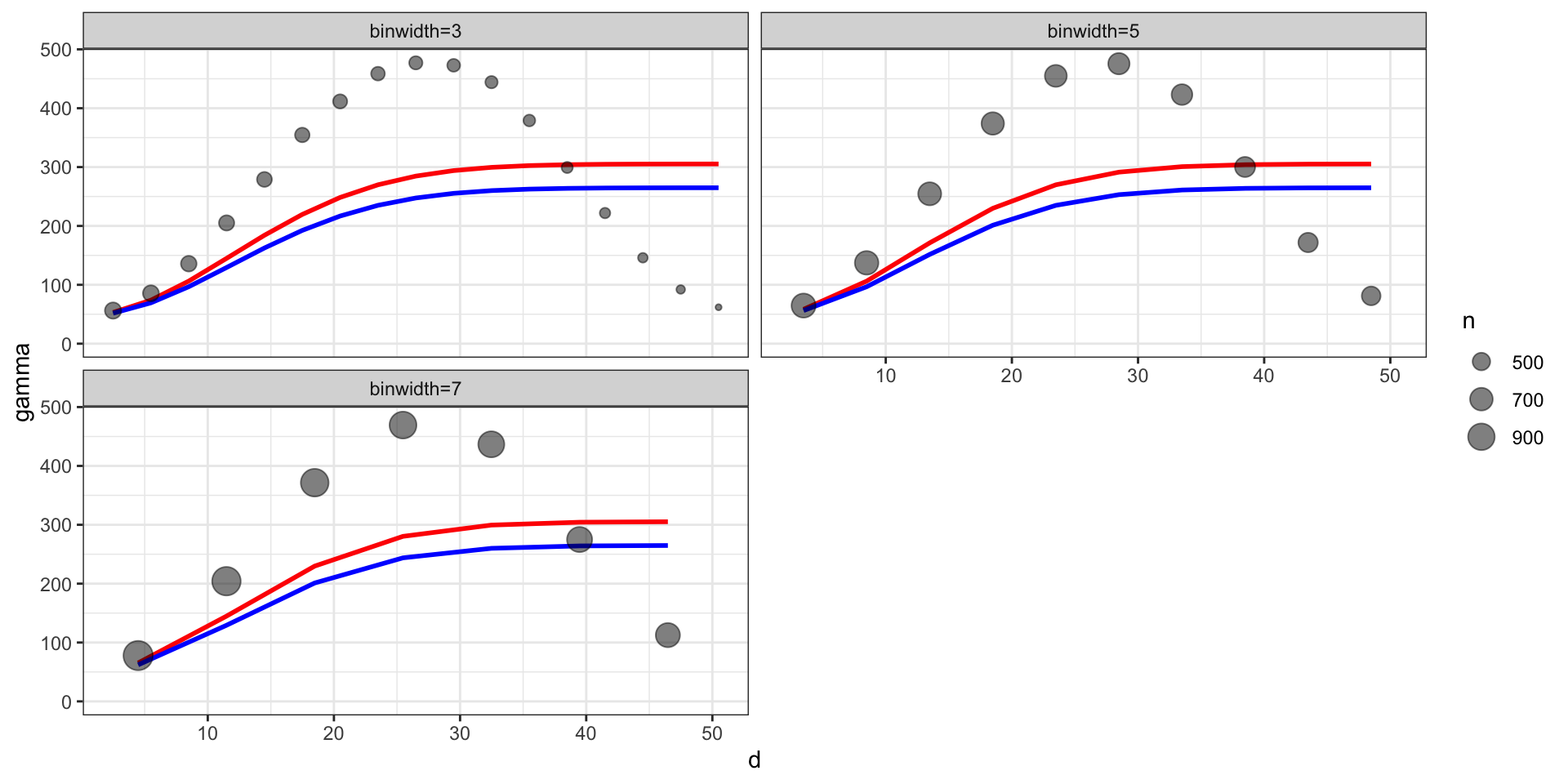
Empirical semivariogram vs. model
From the model summary we have the following,
posterior means: \(\sigma^2 = 258\), \(\sigma^2_w = 47.3\), \(l = 0.06\)
posterior medians: \(\sigma^2 = 218\), \(\sigma^2_w = 46.9\), \(l = 0.06\)
Sta 344 - Fall 2022