Gaussian Process Models

Lecture 14

Dr. Colin Rundel

Multivariate Normal

Multivariate Normal Distribution

For an \(n\)-dimension multivate normal distribution with covariance \(\boldsymbol{\Sigma}\) (positive semidefinite) can be written as

\[ \underset{n \times 1}{\boldsymbol{y}} \sim N(\underset{n \times 1}{\boldsymbol{\mu}}, \; \underset{n \times n}{\boldsymbol{\Sigma}}) \]

\[ \begin{pmatrix} y_1\\ \vdots\\ y_n \end{pmatrix} \sim N\left( \begin{pmatrix} \mu_1\\ \vdots\\ \mu_n \end{pmatrix}, \, \begin{pmatrix} \rho_{11}\sigma_1\sigma_1 & \cdots & \rho_{1n}\sigma_1\sigma_n \\ \vdots & \ddots & \vdots \\ \rho_{n1}\sigma_n\sigma_1 & \cdots & \rho_{nn}\sigma_n\sigma_n \\ \end{pmatrix} \right) \]

Density

For the \(n\) dimensional multivate normal given on the last slide, its density is given by

\[ (2\pi)^{-n/2} \; \det(\boldsymbol{\Sigma})^{-1/2} \; \exp{\left(-\frac{1}{2} \underset{1 \times n}{(\boldsymbol{y}-\boldsymbol{\mu})'} \underset{n \times n}{\boldsymbol{\Sigma}^{-1}} \underset{n \times 1}{(\boldsymbol{y}-\boldsymbol{\mu})}\right)} \]

and its log density is given by

\[ -\frac{n}{2} \log 2\pi - \frac{1}{2} \log \det(\boldsymbol{\Sigma}) - -\frac{1}{2} \underset{1 \times n}{(\boldsymbol{y}-\boldsymbol{\mu})'} \underset{n \times n}{\boldsymbol{\Sigma}^{-1}} \underset{n \times 1}{(\boldsymbol{y}-\boldsymbol{\mu})} \]

Sampling

To generate draws from an \(n\)-dimensional multivate normal with mean \(\underset{n \times 1}{\boldsymbol{\mu}}\) and covariance matrix \(\underset{n \times n}{\boldsymbol{\Sigma}}\),

• Find a matrix \(\underset{n \times n}{\boldsymbol{A}}\) such that \(\boldsymbol{\Sigma} = \boldsymbol{A}\,\boldsymbol{A}^t\)

  • most often we use \(\boldsymbol{A} = \text{Chol}(\boldsymbol{\Sigma})\) where \(\boldsymbol{A}\) is a lower triangular matrix.

• Draw \(n\) iid unit normals, \(N(0,1)\), as \(\underset{n \times 1}{\boldsymbol{z}}\)

• Obtain multivariate normal draws using \[ \underset{n \times 1}{\boldsymbol{y}} = \underset{n \times 1}{\boldsymbol{\mu}} + \underset{n \times n}{\boldsymbol{A}} \, \underset{n \times 1}{\boldsymbol{z}} \]

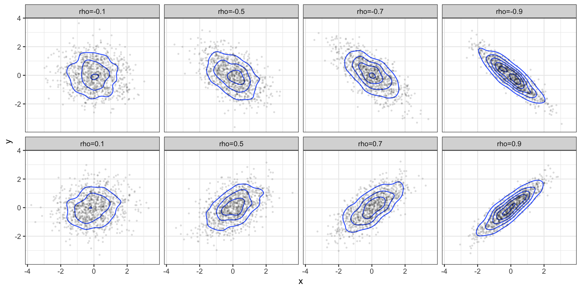
Bivariate Examples

\[ \boldsymbol{\mu} = \begin{pmatrix}0 \\ 0\end{pmatrix} \qquad \boldsymbol{\Sigma} = \begin{pmatrix}1 & \rho \\ \rho & 1 \end{pmatrix}\]

Marginal / conditional distributions

Proposition - For an \(n\)-dimensional multivate normal with mean \(\boldsymbol{\mu}\) and covariance matrix \(\boldsymbol{\Sigma}\), any marginal or conditional distribution of the \(y\)’s will also be (multivariate) normal.

Univariate marginal distribution: \[ y_i = N(\boldsymbol{\mu}_i,\,\boldsymbol{\Sigma}_{ii}) \]

Bivariate marginal distribution: \[ \boldsymbol{y}_{ij} = N\left( \begin{pmatrix}\boldsymbol{\mu}_i \\ \boldsymbol{\mu}_j \end{pmatrix},\; \begin{pmatrix} \boldsymbol{\Sigma}_{ii} & \boldsymbol{\Sigma}_{ij} \\ \boldsymbol{\Sigma}_{ji} & \boldsymbol{\Sigma}_{jj} \end{pmatrix} \right) \]

\(k\)-dimensional marginal distribution:

\[ \boldsymbol{y}_{i,\ldots,k} = N\left( \begin{pmatrix}\boldsymbol{\mu}_{i} \\ \vdots \\ \boldsymbol{\mu}_{k} \end{pmatrix},\; \begin{pmatrix} \boldsymbol{\Sigma}_{ii} & \cdots & \boldsymbol{\Sigma}_{i k} \\ \vdots & \ddots & \vdots \\ \boldsymbol{\Sigma}_{k i} & \cdots & \boldsymbol{\Sigma}_{k k} \end{pmatrix} \right) \]

\(i,\ldots,k\) do not need to be ordered in any particular way

Conditional Distributions

If we partition the \(n\)-dimensions into two pieces such that \(\boldsymbol{y} = (\boldsymbol{y}_1,\, \boldsymbol{y}_2)^t\) then

\[ \underset{n \times 1}{\boldsymbol{y}} \sim N\left( \begin{pmatrix} \boldsymbol{\mu}_1 \\ \boldsymbol{\mu}_2 \end{pmatrix},\, \begin{pmatrix} \boldsymbol{\Sigma}_{11} & \boldsymbol{\Sigma}_{12} \\ \boldsymbol{\Sigma}_{21} & \boldsymbol{\Sigma}_{22} \end{pmatrix} \right) \] \[ \begin{aligned} \underset{k \times 1}{~~\boldsymbol{y}_1~~} &\sim N(\underset{k \times 1}{~~~\boldsymbol{\mu}_1~~~},\, \underset{k \times k}{~~~\boldsymbol{\Sigma}_{11}~~~}) \\ \underset{n-k \times 1}{\boldsymbol{y}_2} &\sim N(\underset{n-k \times 1}{\boldsymbol{\mu}_2},\, \underset{n-k \times n-k}{\boldsymbol{\Sigma}_{22}}) \end{aligned} \]

then the conditional distributions are given by

\[ \begin{aligned} \boldsymbol{y}_1 ~|~ \boldsymbol{y}_2 = \boldsymbol{a} ~&\sim N(\boldsymbol{\mu_1} + \boldsymbol{\Sigma_{12}} \, \boldsymbol{\Sigma_{22}}^{-1} \, (\boldsymbol{a} - \boldsymbol{\mu_2}),~ \boldsymbol{\Sigma_{11}}-\boldsymbol{\Sigma_{12}}\,\boldsymbol{\Sigma_{22}}^{-1} \, \boldsymbol{\Sigma_{21}}) \\ \\ \boldsymbol{y}_2 ~|~ \boldsymbol{y}_1 = \boldsymbol{b} ~&\sim N(\boldsymbol{\mu_2} + \boldsymbol{\Sigma_{21}} \, \boldsymbol{\Sigma_{11}}^{-1} \, (\boldsymbol{b} - \boldsymbol{\mu_1}),~ \boldsymbol{\Sigma_{22}}-\boldsymbol{\Sigma_{21}}\,\boldsymbol{\Sigma_{11}}^{-1} \, \boldsymbol{\Sigma_{12}}) \end{aligned} \]

Gaussian Processes

From Shumway,

A process, \(\boldsymbol{y} = \{y(t) ~:~ t \in T\}\), is said to be a Gaussian process if all possible finite dimensional vectors \(\boldsymbol{y} = (y_{t_1},y_{t_2},...,y_{t_n})^t\), for every collection of time points \(t_1, t_2, \ldots , t_n\), and every positive integer \(n\), have a multivariate normal distribution.

So far we have only looked at examples of time series where \(T\) is discete (and evenly spaces & contiguous), it turns out things get a lot more interesting when we explore the case where \(T\) is defined on a continuous space (e.g. \(\mathbb{R}\) or some subset of \(\mathbb{R}\)).

Gaussian Process Regression

Parameterizing a Gaussian Process

Imagine we have a Gaussian process defined such that \(\boldsymbol{y} = \{y(t) ~:~ t \in [0,1]\}\),

• We now have an uncountably infinite set of possible \(t\)’s and \(y(t)\)s.

• We will only have a (small) finite number of observations \(y(t_1), \ldots, y(t_n)\) with which to say something useful about this infinite dimensional process.

• The unconstrained covariance matrix for the observed data can have up to \(n(n+1)/2\) unique values\(^*\)

• Necessary to make some simplifying assumptions:

  • Stationarity

  • Simple(r) parameterization of \(\Sigma\)

Covariance Functions

More on these next week, but for now some common examples

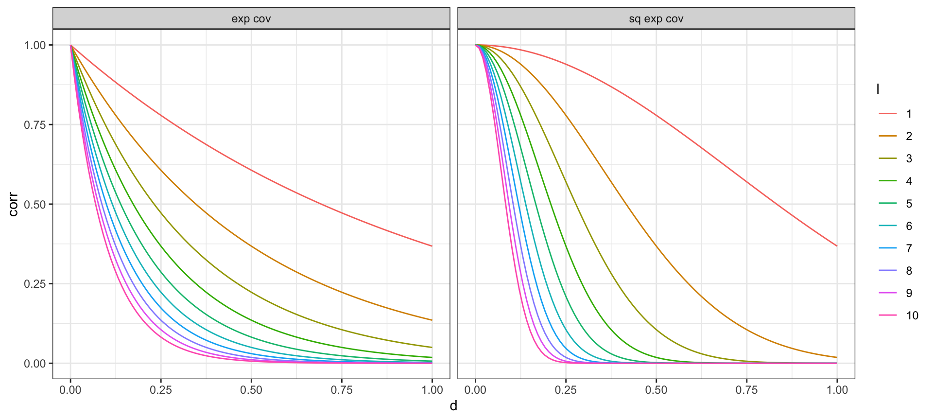
Exponential covariance: \[ \Sigma(y_{t},y_{t'}) = \sigma^2 \exp\big(-|t-t'| \; l\,\big) \]

Squared exponential covariance (Gaussian): \[ \Sigma(y_{t},y_{t'}) = \sigma^2 \exp\big(-(|t-t'| \; l\,)^2\big) \]

Powered exponential covariance \(\left(p \in (0,2]\right)\): \[ \Sigma(y_{t},y_{t'}) = \sigma^2 \exp\big(-(|t-t'| \; l\,)^p\big) \]

Covariance Function - Correlation Decay

Letting \(\sigma^2 = 1\) and trying different values of the length scale \(l\),

Correlation Decay - AR(1)

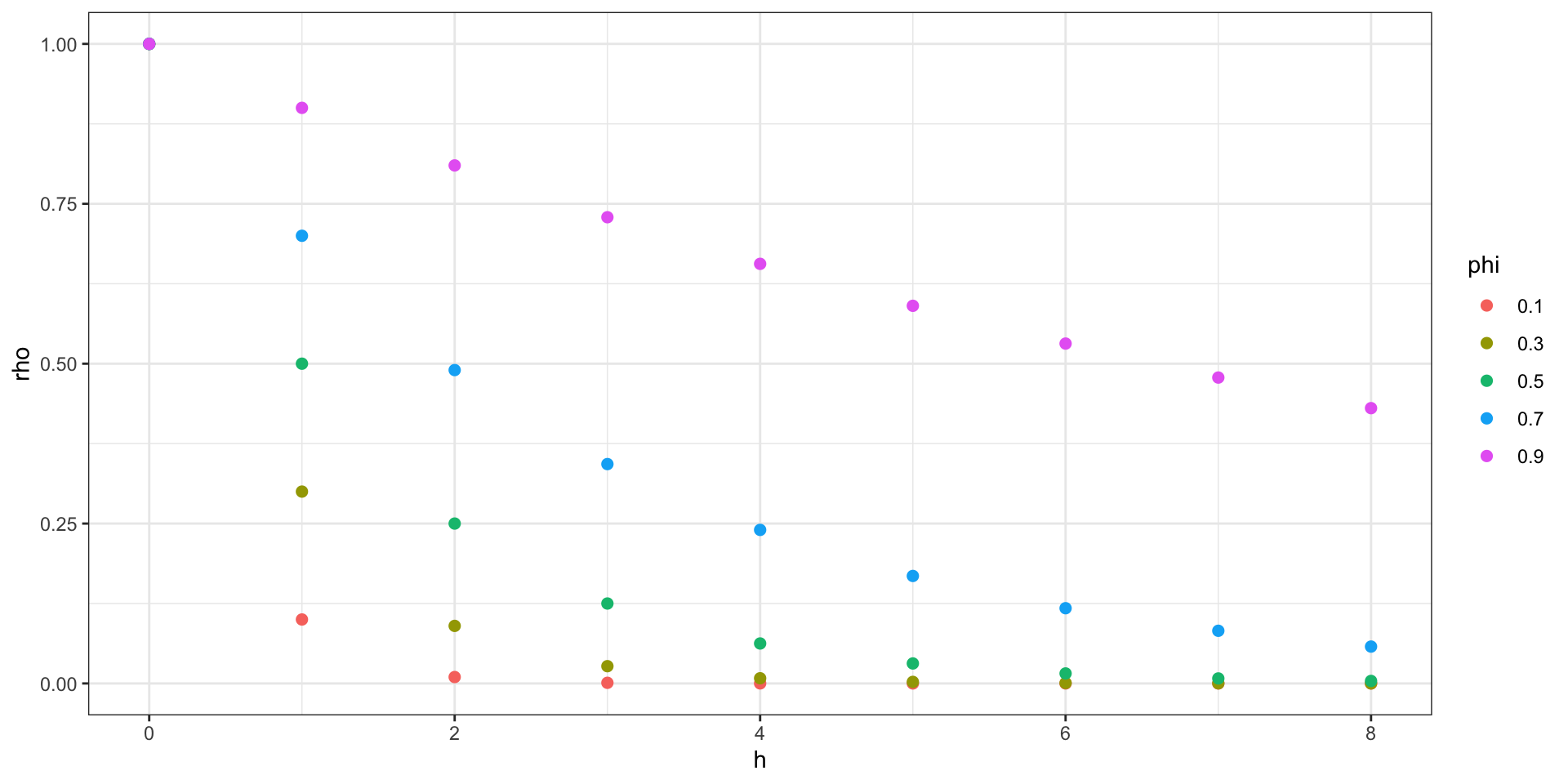
Recall that for a stationary AR(1) process: \(\gamma(h) = \sigma^2_w \phi^{|h|}\) and \(\rho(h) = \phi^{|h|}\)

we can draw a somewhat similar picture about the decay of \(\rho\) as a function of distance.

Example

Prediction

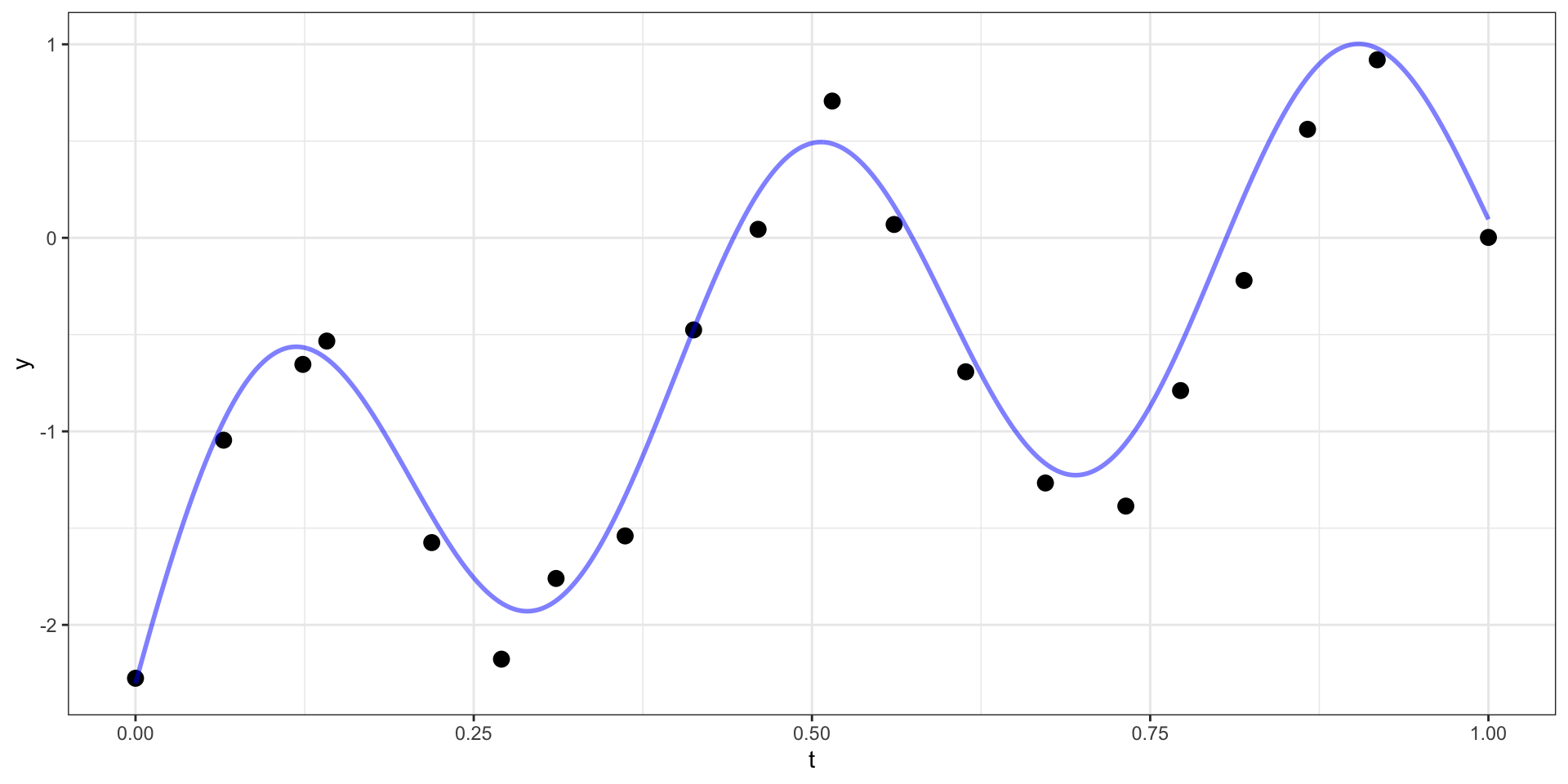
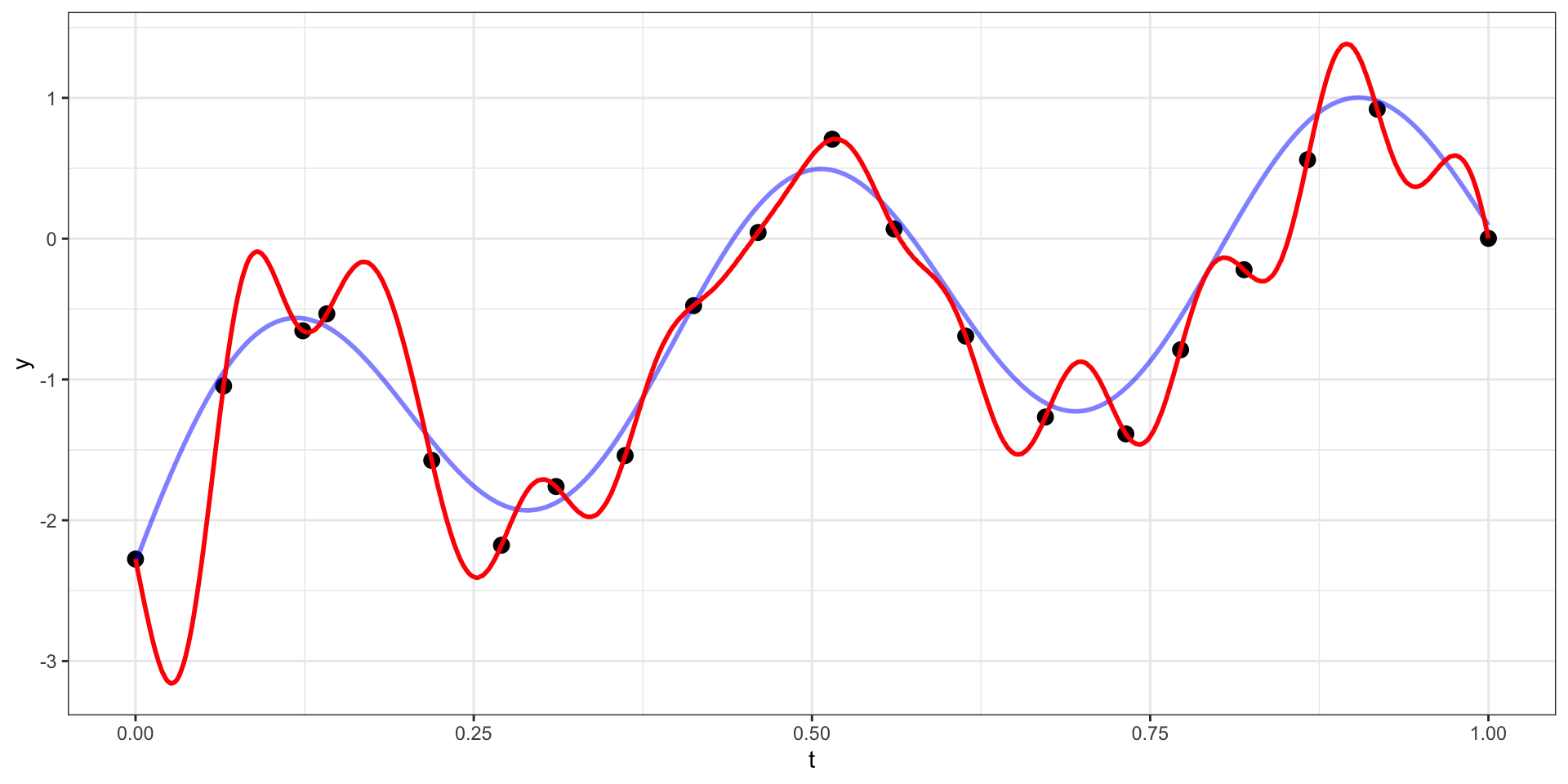
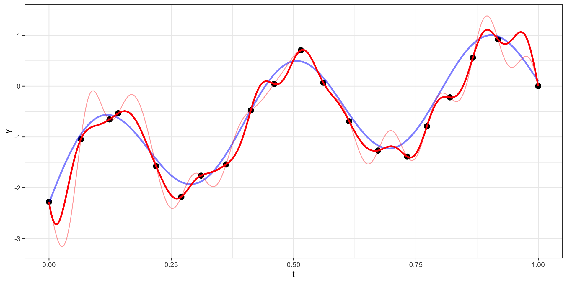
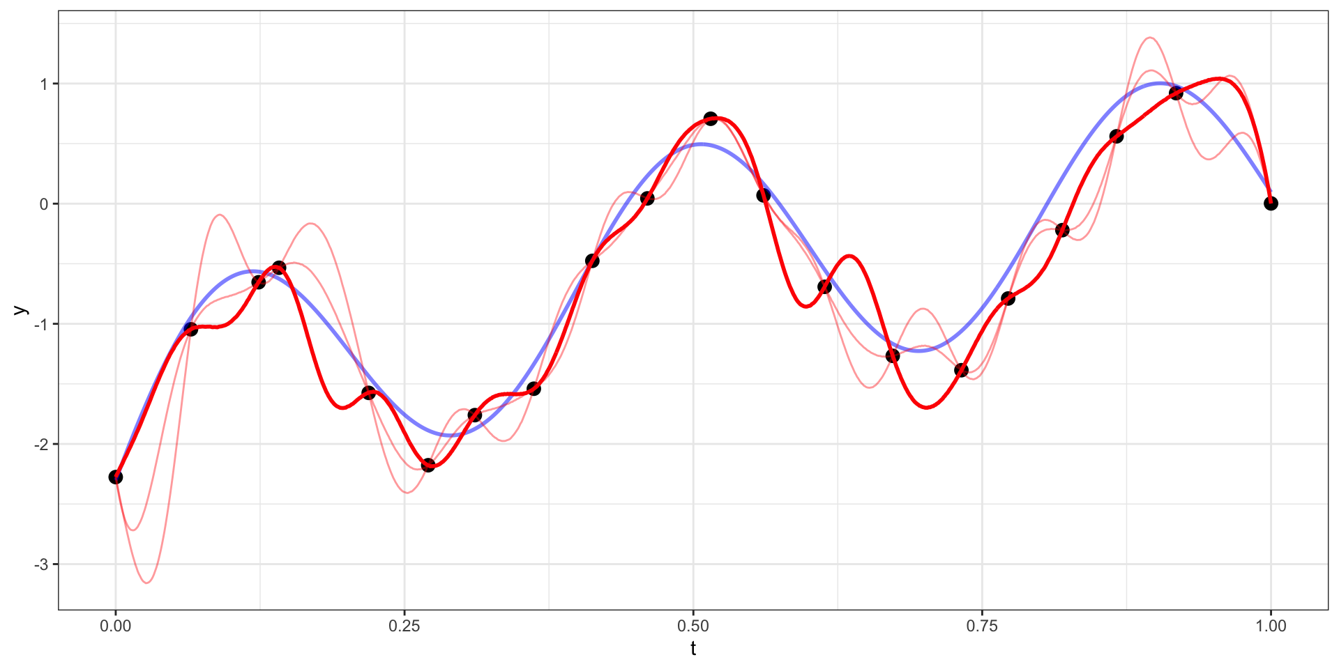
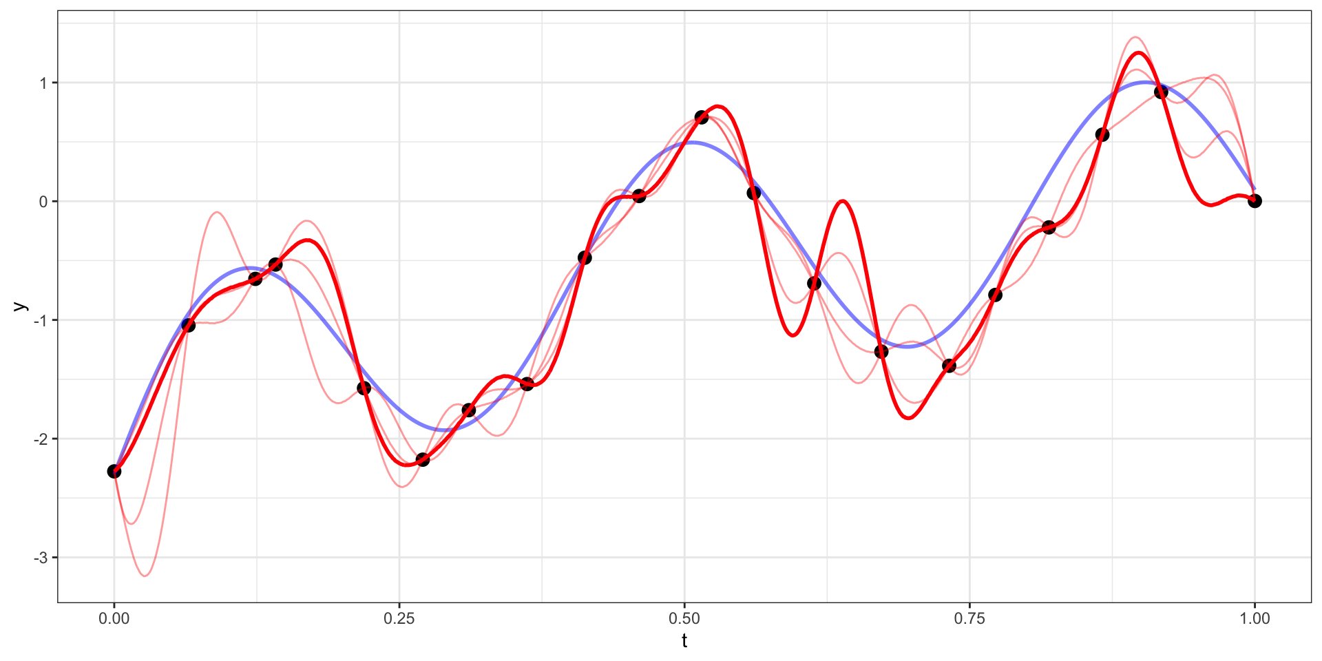
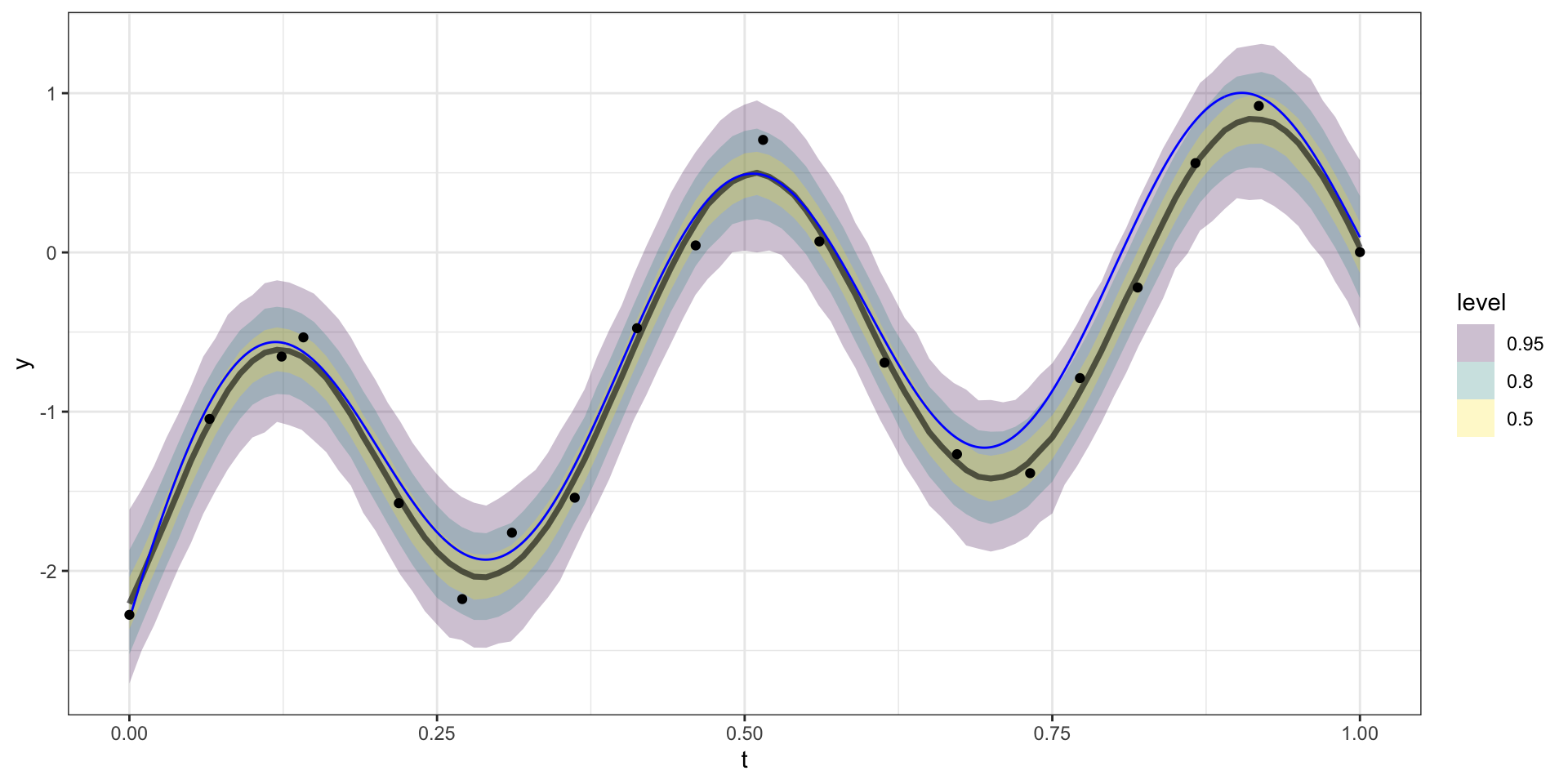
Our example has 20 observations which we would like to use as the basis for predicting \(y(t)\) at other values of \(t\) (say a regular sequence of values from 0 to 1).

For now lets use a square exponential covariance with \(\sigma^2 = 10\) and \(l=15\)

We therefore want to sample from \(\boldsymbol{y}_{pred} | \boldsymbol{y}_{obs}\).

\[\boldsymbol{y}_{pred} ~|~ \boldsymbol{y}_{obs} = \boldsymbol{y} ~\sim N(\boldsymbol{\Sigma}_{po} \, \boldsymbol{\Sigma}_{obs}^{-1} \, \boldsymbol{y},~ \boldsymbol{\Sigma}_{pred}-\boldsymbol{\Sigma}_{po}\,\boldsymbol{\Sigma}_{pred}^{-1} \, \boldsymbol{\Sigma}_{op})\]

Draw 1

Draw 2

Draw 3

Draw 4

Draw 5

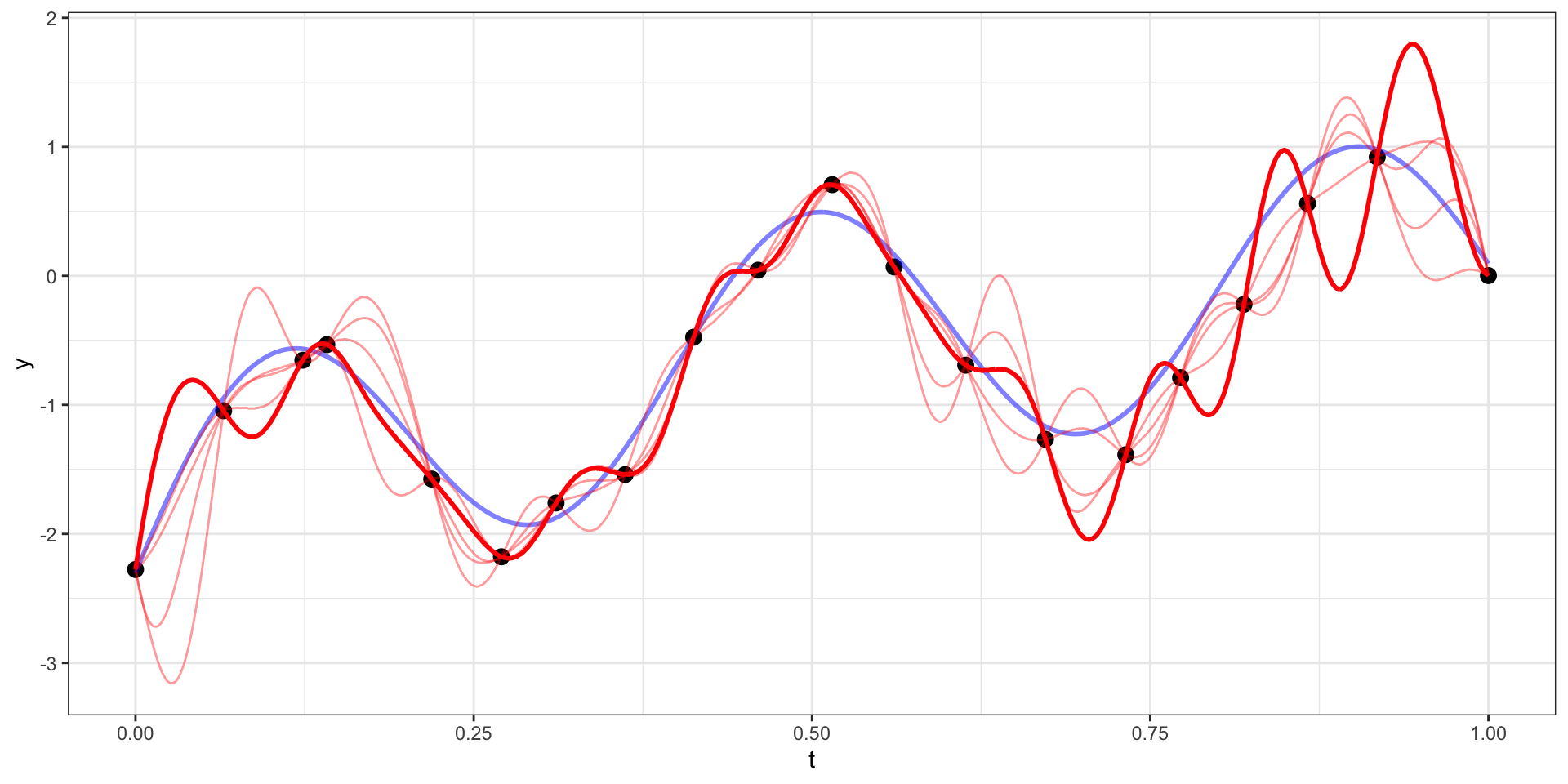
Many draws later

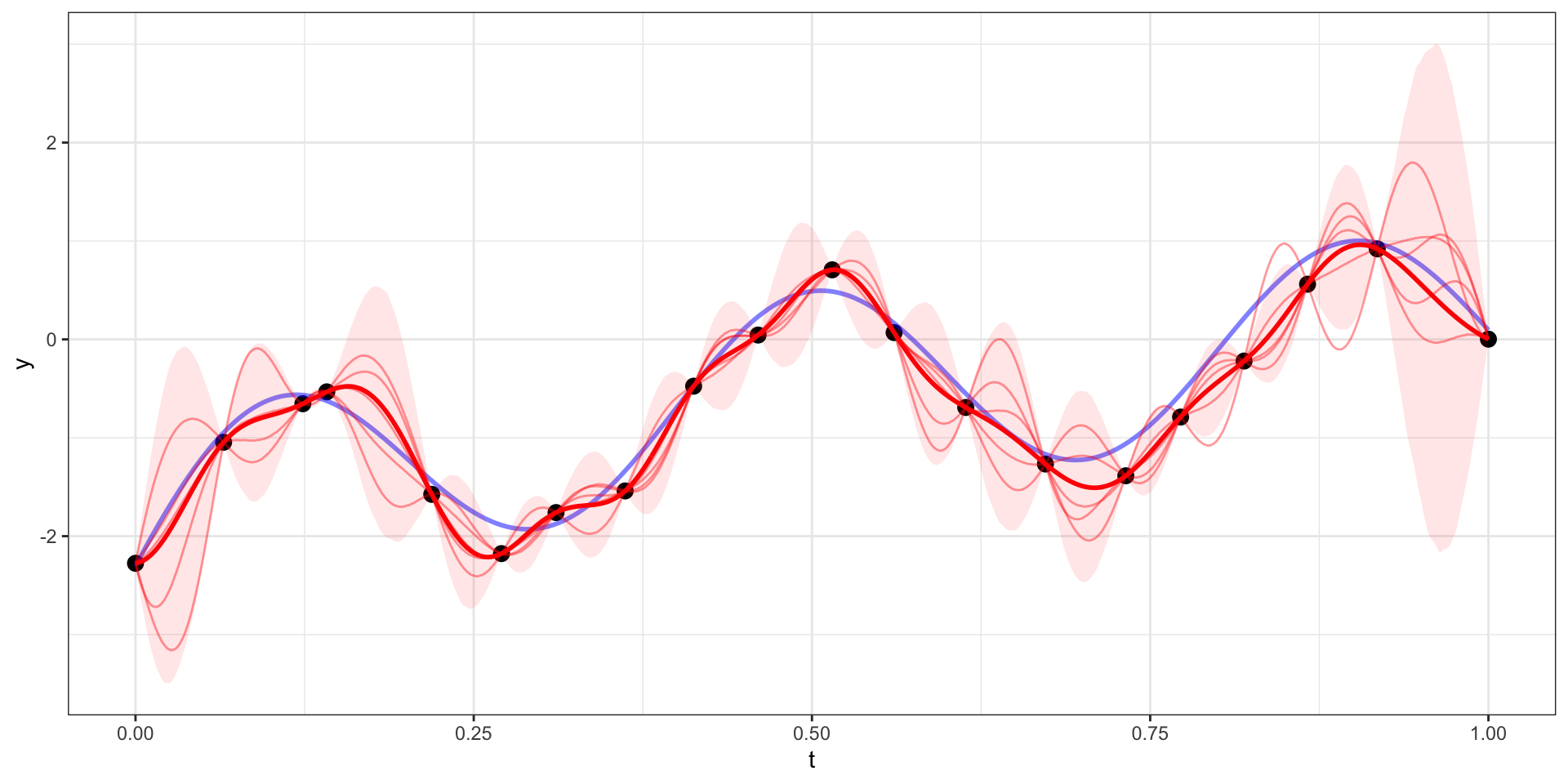
Exponential Covariance

Where \(\sigma=10\), \(l = \sqrt{15}\),

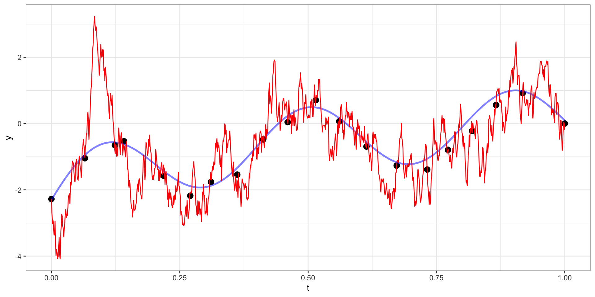
Exponential Covariance - Draw 2

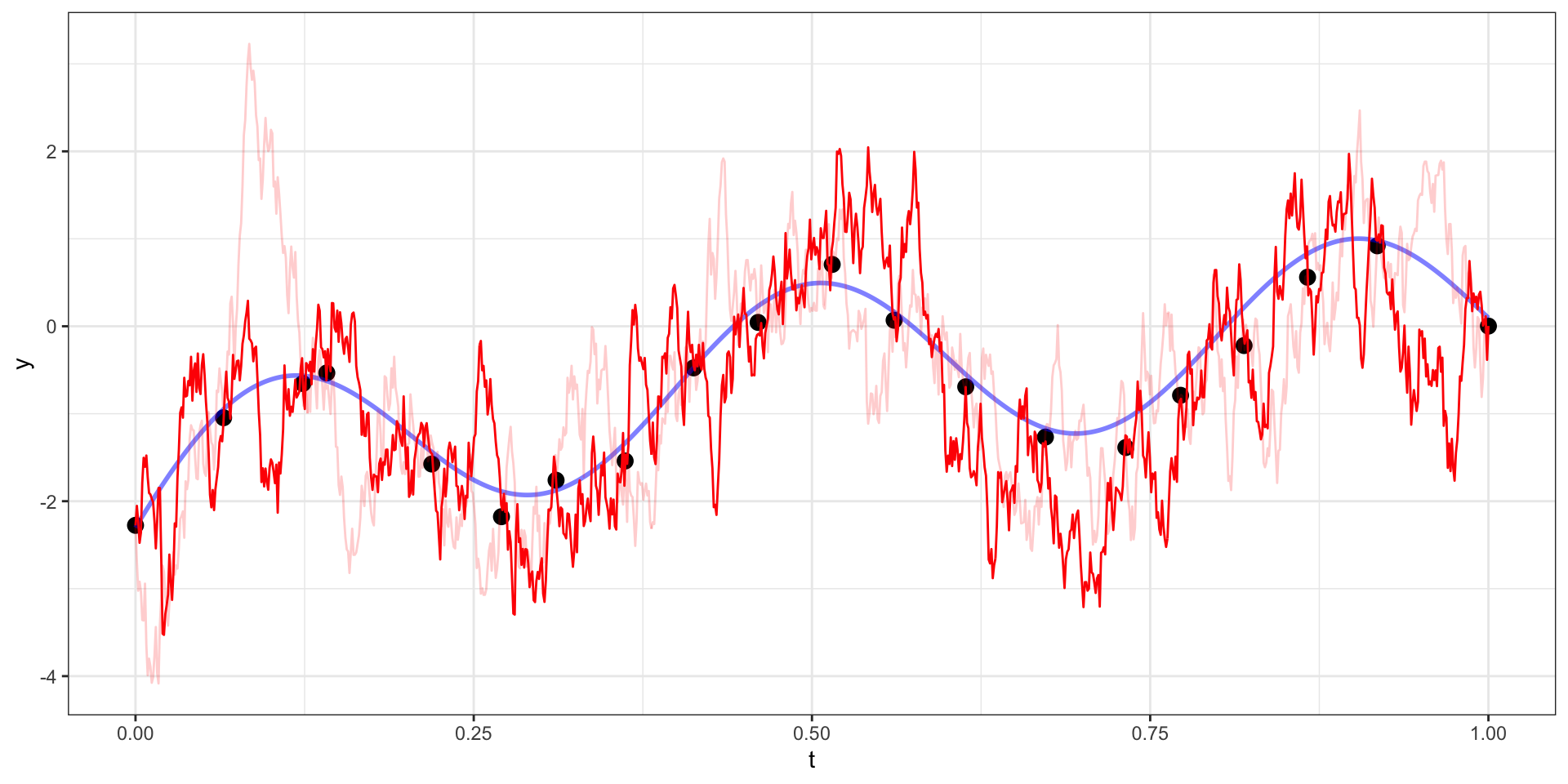
Exponential Covariance - Draw 3

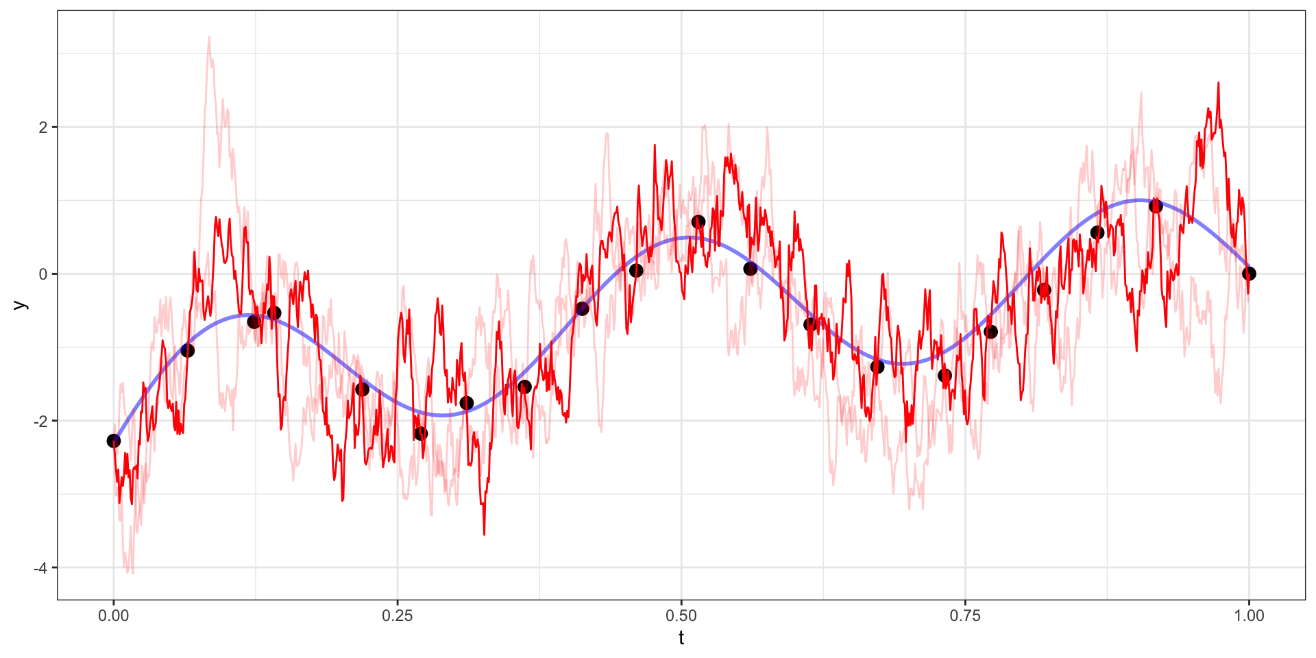
Exponential Covariance - Draw 4

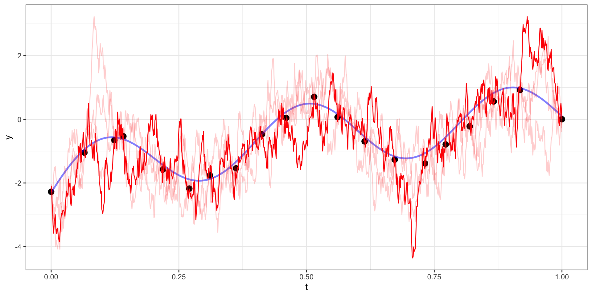
Exponential Covariance - Draw 5

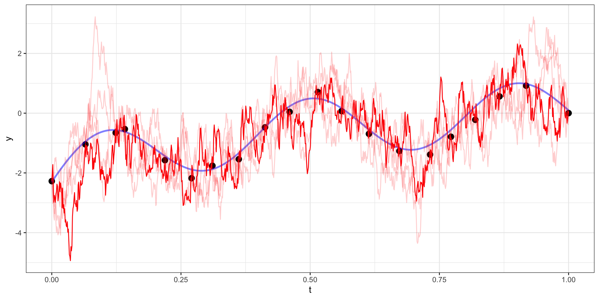
Exponential Covariance - Variability

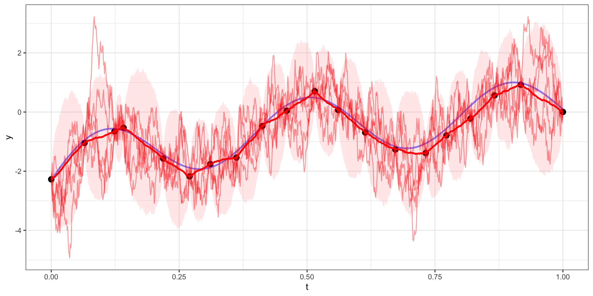
Powered Exponential Covariance (\(p=1.5\))

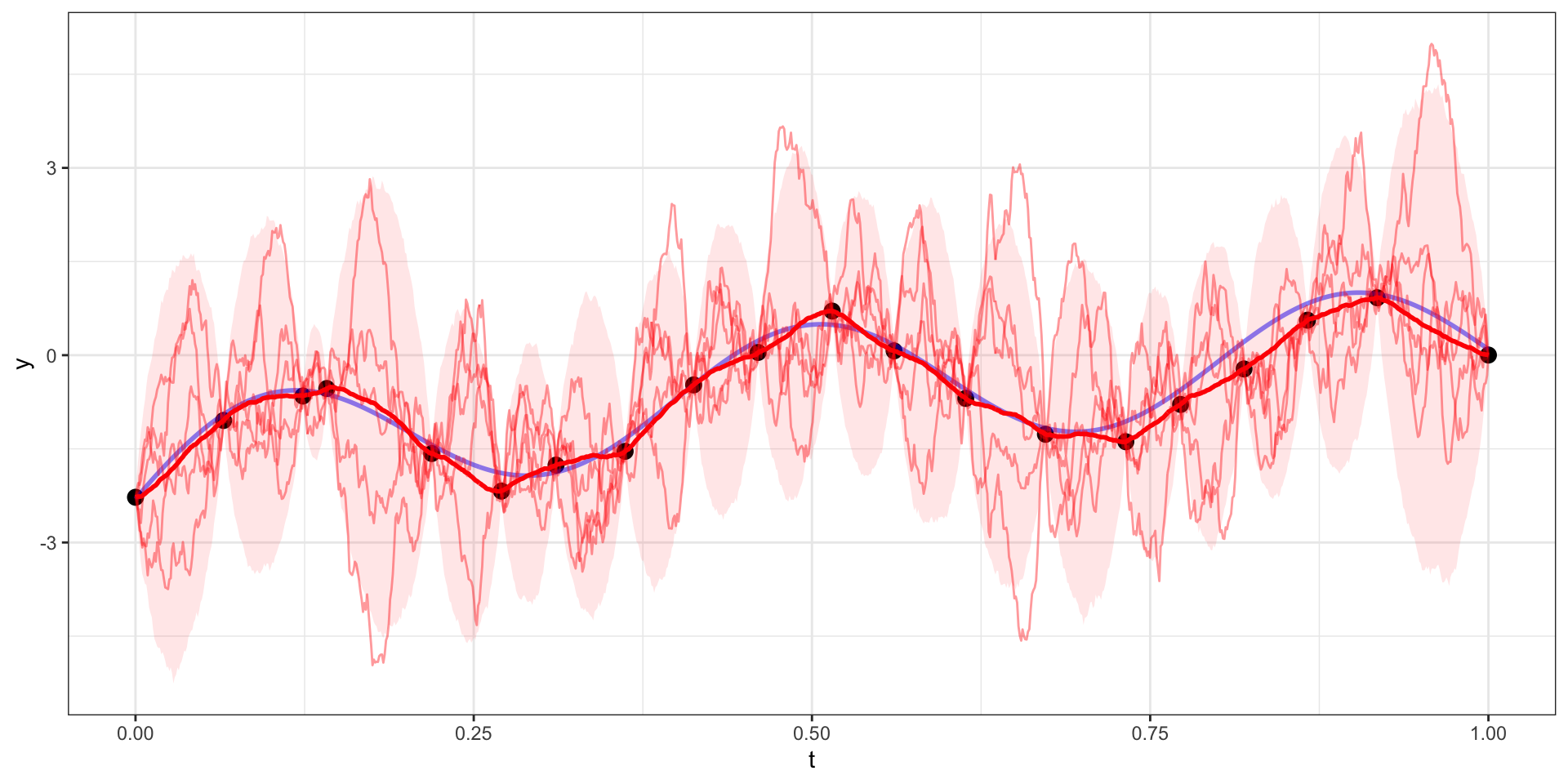
Back to the square exponential

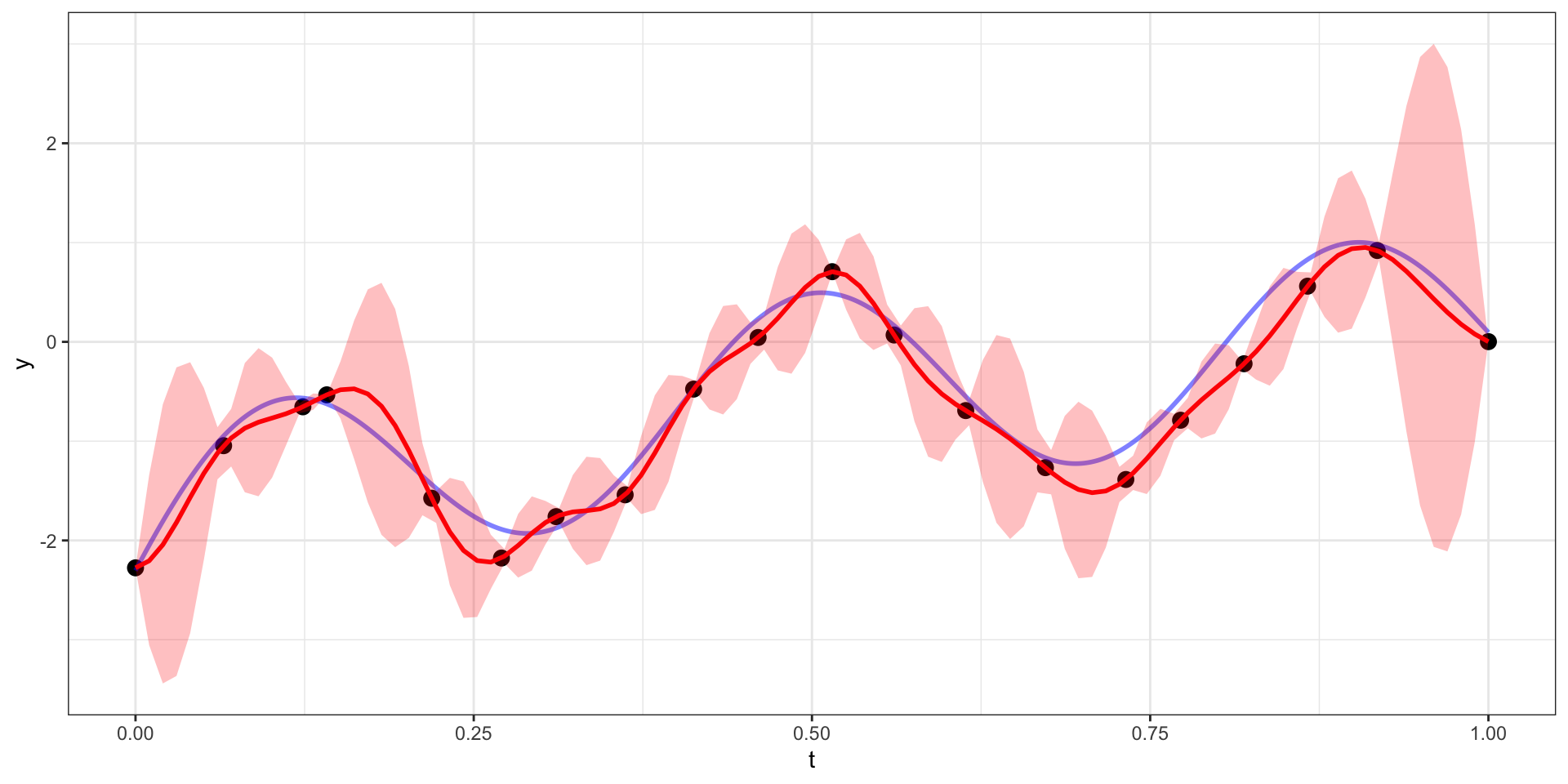
Changing the range (\(l\))

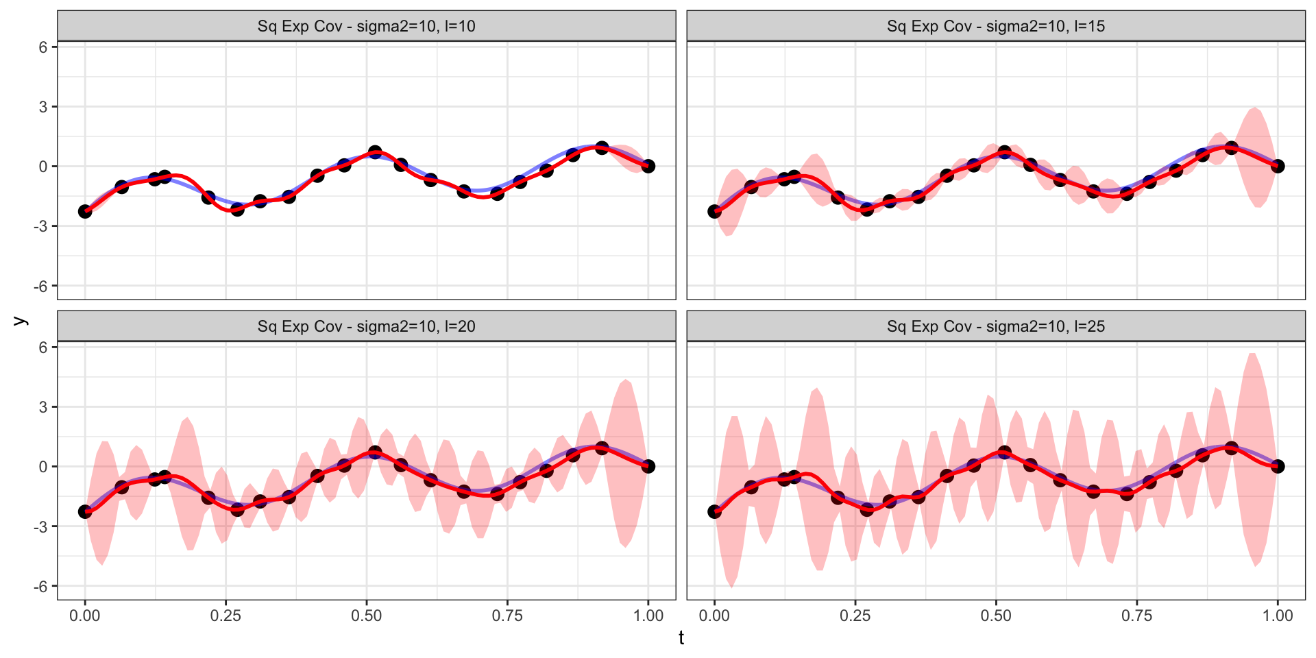
Effective Range

For the square exponential covariance \[ \begin{aligned} Cov(d) &= \sigma^2 \exp\left(-(l \cdot d)^2\right) \\ Corr(d) &= \exp\left(-(l \cdot d)^2\right) \end{aligned} \]

we would like to know, for a given value of \(l\), beyond what distance apart must observations be to have a correlation less than \(0.05\)?

\[ \begin{aligned} \exp\left(-(l \cdot d)^2\right) &< 0.05 \\ -(l \cdot d)^2 &< \log 0.05 \\ l \cdot d &< \sqrt{3} \\ d &< \sqrt{3} / l \end{aligned} \]

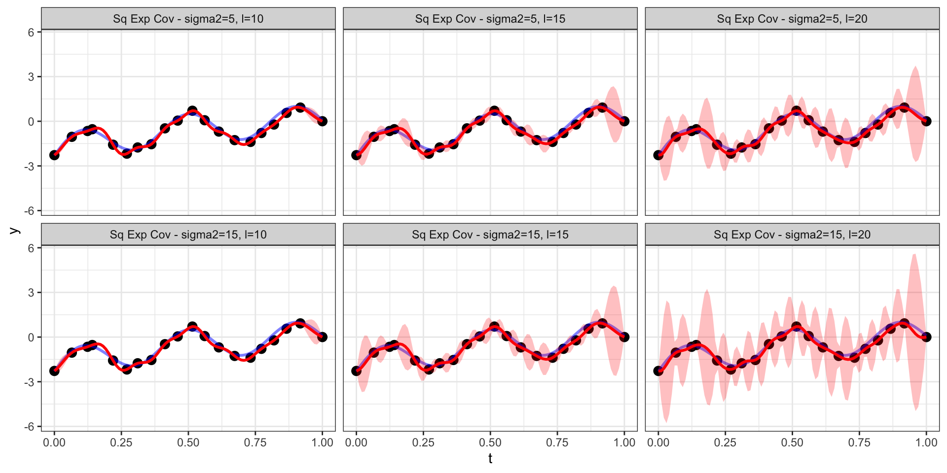
Changing the scale (\(\sigma^2\))

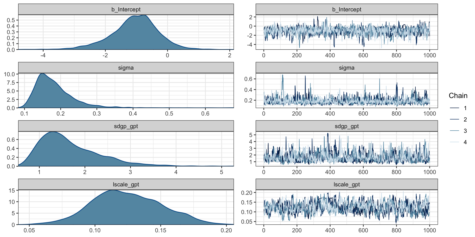
Fitting w/ BRMS

library(brms)
gp = brm(y ~ gp(t), data=d, cores=4, refresh=0)

summary(gp)

 Family: gaussian 
  Links: mu = identity; sigma = identity 
Formula: y ~ gp(t) 
   Data: d (Number of observations: 20) 
  Draws: 4 chains, each with iter = 2000; warmup = 1000; thin = 1;
         total post-warmup draws = 4000

Gaussian Process Terms: 
            Estimate Est.Error l-95% CI u-95% CI
sdgp(gpt)       1.67      0.67     0.79     3.31
lscale(gpt)     0.12      0.03     0.08     0.18
            Rhat Bulk_ESS Tail_ESS
sdgp(gpt)   1.01      390     1098
lscale(gpt) 1.02      262      316

Population-Level Effects: 
          Estimate Est.Error l-95% CI u-95% CI
Intercept    -1.07      0.79    -2.80     0.36
          Rhat Bulk_ESS Tail_ESS
Intercept 1.01     1065     1131

Family Specific Parameters: 
      Estimate Est.Error l-95% CI u-95% CI Rhat
sigma     0.18      0.06     0.11     0.32 1.00
      Bulk_ESS Tail_ESS
sigma      914     1180

Draws were sampled using sampling(NUTS). For each parameter, Bulk_ESS
and Tail_ESS are effective sample size measures, and Rhat is the potential
scale reduction factor on split chains (at convergence, Rhat = 1).

Trace plots

plot(gp)

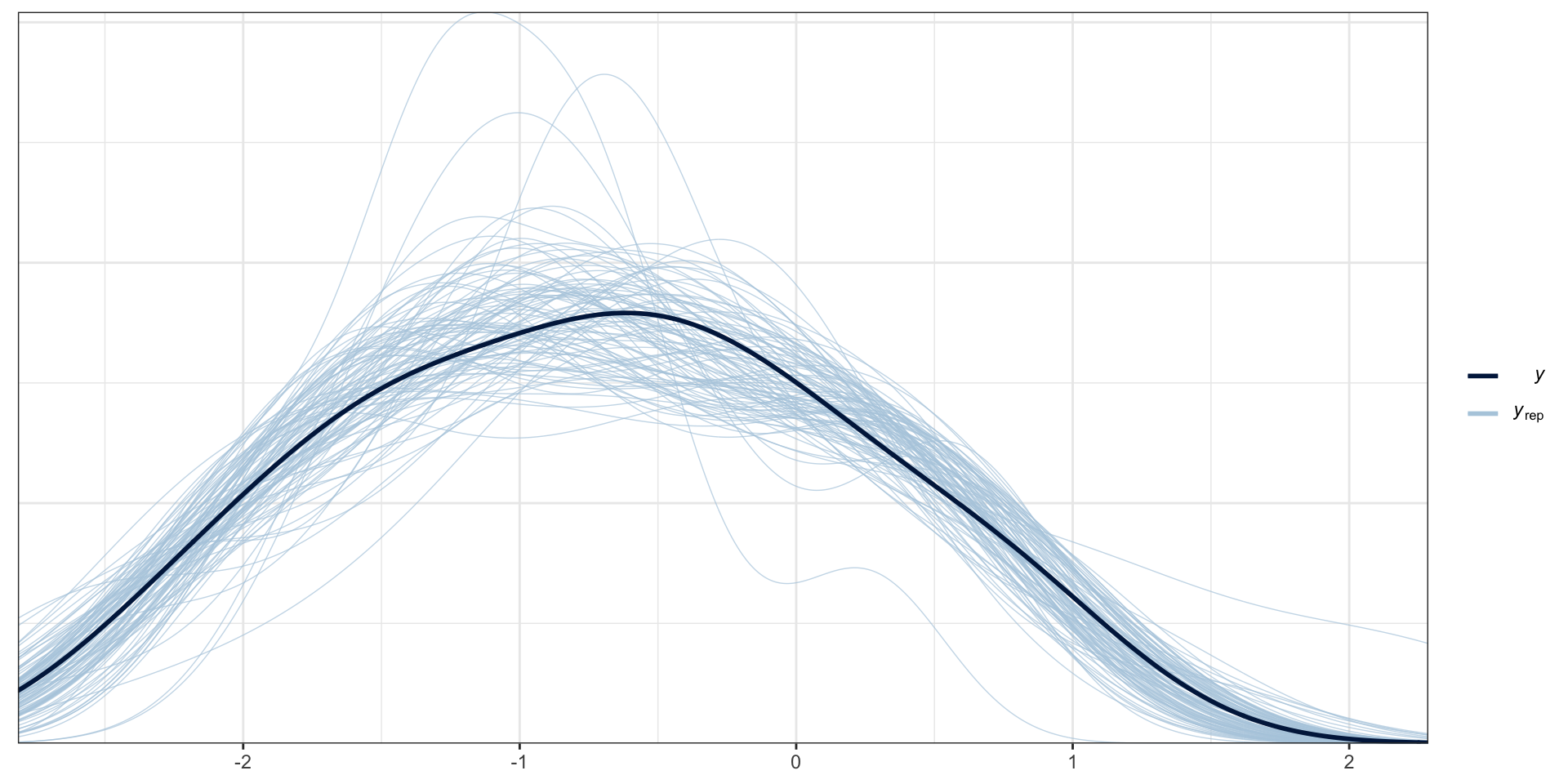
PP Checks

pp_check(gp, ndraws = 100)

Model predictions

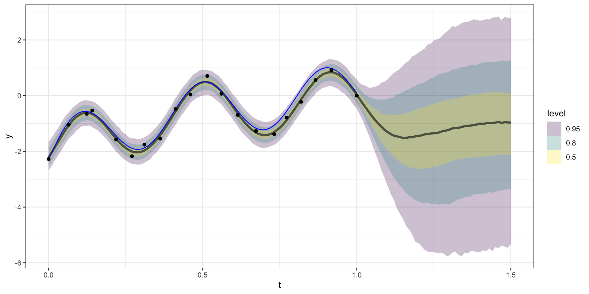
Forecasting

Stan code

gp %>%
  brms::stancode()

// generated with brms 2.18.0
functions {
  /* compute a latent Gaussian process
   * Args:
   *   x: array of continuous predictor values
   *   sdgp: marginal SD parameter
   *   lscale: length-scale parameter
   *   zgp: vector of independent standard normal variables
   * Returns:
   *   a vector to be added to the linear predictor
   */
  vector gp(data vector[] x, real sdgp, vector lscale, vector zgp) {
    int Dls = rows(lscale);
    int N = size(x);
    matrix[N, N] cov;
    if (Dls == 1) {
      // one dimensional or isotropic GP
      cov = gp_exp_quad_cov(x, sdgp, lscale[1]);
    } else {
      // multi-dimensional non-isotropic GP
      cov = gp_exp_quad_cov(x[, 1], sdgp, lscale[1]);
      for (d in 2:Dls) {
        cov = cov .* gp_exp_quad_cov(x[, d], 1, lscale[d]);
      }
    }
    for (n in 1:N) {
      // deal with numerical non-positive-definiteness
      cov[n, n] += 1e-12;
    }
    return cholesky_decompose(cov) * zgp;
  }
  /* Spectral density function of a Gaussian process
   * with squared exponential covariance kernel
   * Args:
   *   x: array of numeric values of dimension NB x D
   *   sdgp: marginal SD parameter
   *   lscale: vector of length-scale parameters
   * Returns:
   *   numeric values of the function evaluated at 'x'
   */
  vector spd_cov_exp_quad(data vector[] x, real sdgp, vector lscale) {
    int NB = dims(x)[1];
    int D = dims(x)[2];
    int Dls = rows(lscale);
    vector[NB] out;
    if (Dls == 1) {
      // one dimensional or isotropic GP
      real constant = square(sdgp) * (sqrt(2 * pi()) * lscale[1])^D;
      real neg_half_lscale2 = -0.5 * square(lscale[1]);
      for (m in 1:NB) {
        out[m] = constant * exp(neg_half_lscale2 * dot_self(x[m]));
      }
    } else {
      // multi-dimensional non-isotropic GP
      real constant = square(sdgp) * sqrt(2 * pi())^D * prod(lscale);
      vector[Dls] neg_half_lscale2 = -0.5 * square(lscale);
      for (m in 1:NB) {
        out[m] = constant * exp(dot_product(neg_half_lscale2, square(x[m])));
      }
    }
    return out;
  }
  /* how many elements are in a range of integers?
   * Args:
   *   x: an integer array
   *   start: start of the range (inclusive)
   *   end: end of the range (inclusive)
   * Returns:
   *   a scalar integer
   */
  int size_range(int[] x, int start, int end) {
    int out = 0;
    for (i in 1:size(x)) {
      out += (x[i] >= start && x[i] <= end);
    }
    return out;
  }
  /* which elements are in a range of integers?
   * Args:
   *   x: an integer array
   *   start: start of the range (inclusive)
   *   end: end of the range (inclusive)
   * Returns:
   *   an integer array
   */
  int[] which_range(int[] x, int start, int end) {
    int out[size_range(x, start, end)];
    int j = 1;
    for (i in 1:size(x)) {
      if (x[i] >= start && x[i] <= end) {
        out[j] = i;
        j += 1;
      }
    }
    return out;
  }
  /* adjust array values to x - start + 1
   * Args:
   *   x: an integer array
   *   start: start of the range of values in x (inclusive)
   * Returns:
   *   an integer array
   */
  int[] start_at_one(int[] x, int start) {
    int out[size(x)];
    for (i in 1:size(x)) {
      out[i] = x[i] - start + 1;
    }
    return out;
  }
}
data {
  int<lower=1> N;  // total number of observations
  vector[N] Y;  // response variable
  // data related to GPs
  int<lower=1> Kgp_1;  // number of sub-GPs (equal to 1 unless 'by' was used)
  int<lower=1> Dgp_1;  // GP dimension
  // number of latent GP groups
  int<lower=1> Nsubgp_1;
  // indices of latent GP groups per observation
  int<lower=1> Jgp_1[N];
  vector[Dgp_1] Xgp_1[Nsubgp_1];  // covariates of the GP
  int prior_only;  // should the likelihood be ignored?
}
transformed data {
}
parameters {
  real Intercept;  // temporary intercept for centered predictors
  vector<lower=0>[Kgp_1] sdgp_1;  // GP standard deviation parameters
  vector<lower=0>[1] lscale_1[Kgp_1];  // GP length-scale parameters
  vector[Nsubgp_1] zgp_1;  // latent variables of the GP
  real<lower=0> sigma;  // dispersion parameter
}
transformed parameters {
  real lprior = 0;  // prior contributions to the log posterior
  lprior += student_t_lpdf(Intercept | 3, -0.7, 2.5);
  lprior += student_t_lpdf(sdgp_1 | 3, 0, 2.5)
    - 1 * student_t_lccdf(0 | 3, 0, 2.5);
  lprior += inv_gamma_lpdf(lscale_1[1][1] | 1.82247, 0.11151);
  lprior += student_t_lpdf(sigma | 3, 0, 2.5)
    - 1 * student_t_lccdf(0 | 3, 0, 2.5);
}
model {
  // likelihood including constants
  if (!prior_only) {
    vector[Nsubgp_1] gp_pred_1 = gp(Xgp_1, sdgp_1[1], lscale_1[1], zgp_1);
    // initialize linear predictor term
    vector[N] mu = rep_vector(0.0, N);
    mu += Intercept + gp_pred_1[Jgp_1];
    target += normal_lpdf(Y | mu, sigma);
  }
  // priors including constants
  target += lprior;
  target += std_normal_lpdf(zgp_1);
}
generated quantities {
  // actual population-level intercept
  real b_Intercept = Intercept;
}