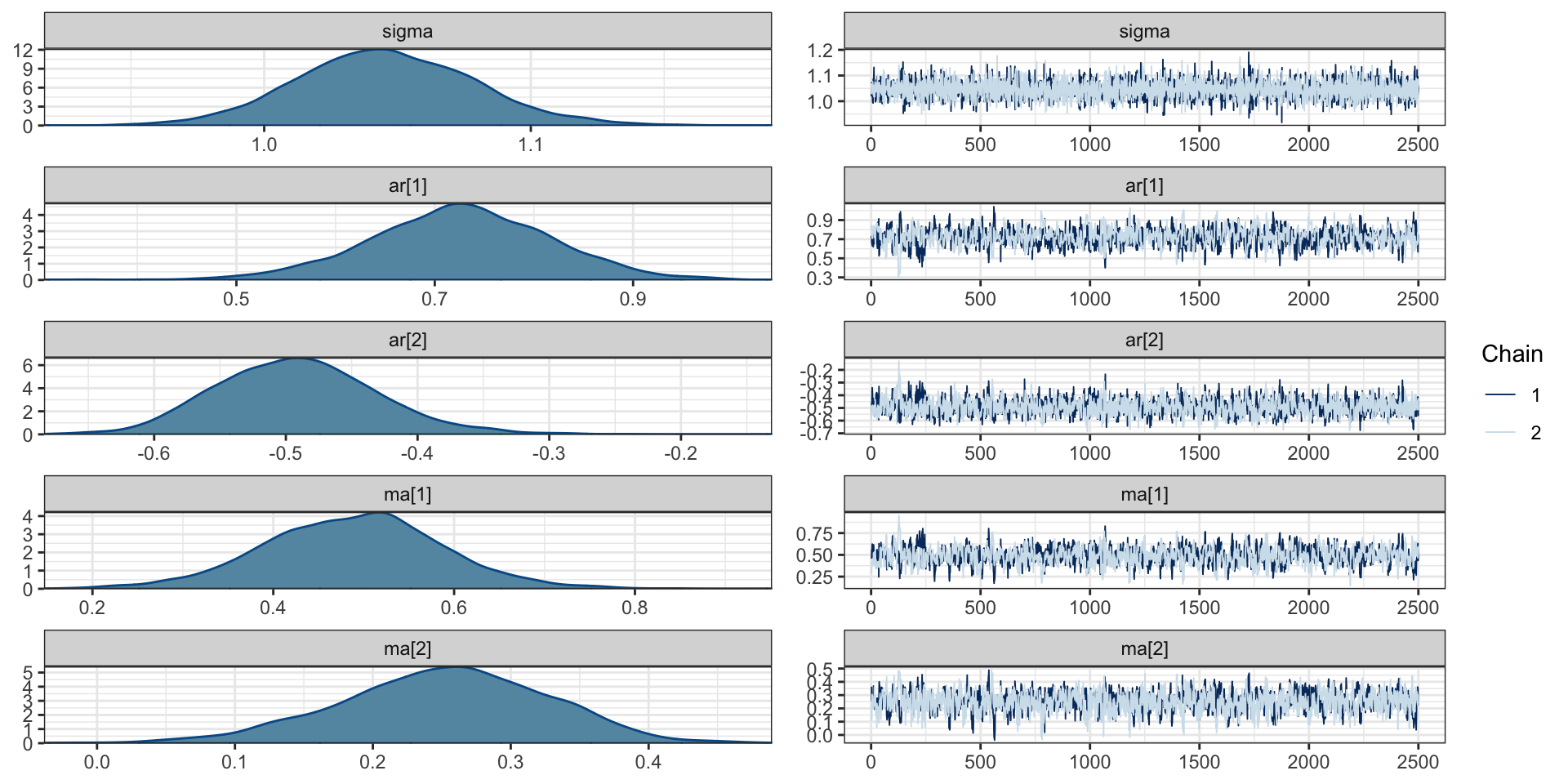
Series: ar1
ARIMA(1,0,0) with non-zero mean

Coefficients:
         ar1    mean
      0.7601  2.2178
s.e.  0.0290  0.1890

sigma^2 = 1.045:  log likelihood = -719.84
AIC=1445.67 AICc=1445.72 BIC=1458.32Fitting ARIMA Models
Lecture 12
Model Fitting
Fitting ARIMA
For an \(ARIMA(p,d,q)\) model,
Assumes that the data is stationary after differencing
Handling \(d\) is straight forward, just difference the original data \(d\) times (leaving \(n-d\) observations) \[ y'_t = \Delta^d \, y_t \]
After differencing, fit an \(ARMA(p,q)\) model to \(y'_t\).
To keep things simple we’ll assume \(w_t \overset{iid}{\sim} \mathcal{N}(0,\sigma^2_w)\)
MLE - Stationarity & iid normal errors
If both of these assumptions are met, then the time series \(y_t\) will also be normal.
In general, the vector \(\boldsymbol{y} = (y_1, y_2, \ldots, y_t)'\) will have a multivariate normal distribution with mean \(\{\boldsymbol\mu\}_i = E(y_i) = E(y_t)\) and covariance \(\boldsymbol\Sigma\) where \(\{\boldsymbol{\Sigma}\}_{ij} = \gamma(i-j)\).
The joint density of \(\boldsymbol y\) is given by
\[ f_{\boldsymbol y}(\boldsymbol y) = \frac{1}{(2\pi)^{t/2}\,\det(\boldsymbol\Sigma)^{1/2}} \times \exp\left( -\frac{1}{2}(\boldsymbol y - \boldsymbol \mu)' \, \Sigma^{-1} \, (\boldsymbol y - \boldsymbol \mu) \right) \]
AR
Fitting \(AR(1)\)
\[ y_t = \delta + \phi \, y_{t-1} + w_t \]
We need to estimate three parameters: \(\delta\), \(\phi\), and \(\sigma_w^2\), we know
\[ \begin{aligned} E(y_t) = \frac{\delta}{1-\phi} \quad&\quad Var(y_t) = \frac{\sigma_w^2}{1-\phi^2} \\ \gamma(h) &= \frac{\sigma_w^2}{1-\phi^2} \phi^{|h|} \end{aligned} \]
Using these properties it is possible to write the distribution of \(\boldsymbol{y}\) as a MVN but that does not make it easy to write down a (simplified) closed form for the MLE estimate for \(\delta\), \(\phi\), and \(\sigma_w^2\).
Conditional Density
We can also rewrite the density as follows,
\[ \begin{aligned} f(\boldsymbol y) &= f(y_t,\,y_{t-1},\,\ldots,\,y_2,\,y_1) \\ &= f(y_t|\,y_{t-1},\,\ldots,\,y_2,\,y_1) f(y_{t-1}|y_{t-2},\,\ldots,\,y_2,\,y_1) \cdots f(y_2|y_1) f(y_1) \\ &= f(y_t|\,y_{t-1}) f(y_{t-1}|y_{t-2}) \cdots f(y_2|y_1) f(y_1) \end{aligned} \]
where,
\[ \begin{aligned} y_1 &\sim \mathcal{N}\left(\delta, \, \frac{\sigma^2_w}{1-\phi^2} \right) \\ y_{t}|y_{t-1} &\sim \mathcal{N}\left(\delta+\phi\, y_{t-1}, \, \sigma^2_w \right) \\ f(y_{t}|y_{t-1}) &= \frac{1}{\sqrt{2\pi \, \sigma^2_w}} \exp \left( -\frac{1}{2}\frac{(y_t -\delta+\phi\, y_{t-1})^2 }{\sigma^2_w} \right) \end{aligned} \]
Log likelihood of AR(1)
\[ \log f(y_{t} | y_{t-1}) = -\frac{1}{2}\left( \log 2\pi + \log \sigma^2_w + \frac{1}{\sigma_w^2} (y_t -\delta+\phi\, y_{t-1})^2 \right) \]
\[ \begin{aligned} \ell(\delta, \phi, \sigma^2_w) &= \log f(\boldsymbol{y}) = \log f(y_1) + \sum_{i=2}^t \log f(y_{i}|y_{i-1}) \\ &= - \frac{1}{2} \bigg(\log 2\pi + \log \sigma_w^2 - \log (1-\phi^2) + \frac{(1-\phi^2)}{\sigma_w^2 }(y_1-\delta)^2 \bigg) \\ & ~~~~ - \frac{1}{2} \bigg( (n-1) \log 2\pi + (n-1) \log \sigma_w^2 + \frac{1}{\sigma_w^2} \sum_{i=2}^n (y_i -\delta+\phi\, y_{i-1})^2 \bigg) \\ &= - \frac{1}{2} \bigg( n \log 2\pi + n \log \sigma_w^2 - \log (1-\phi^2) \\ &~~~~~~~~~~~~~~~+ \frac{1}{\sigma_w^2} \bigg( (1-\phi^2)(y_1-\delta)^2 + \sum_{i=2}^n (y_i -\delta+\phi\, y_{i-1})^2 \bigg) \bigg) \end{aligned} \]
AR(1) Example
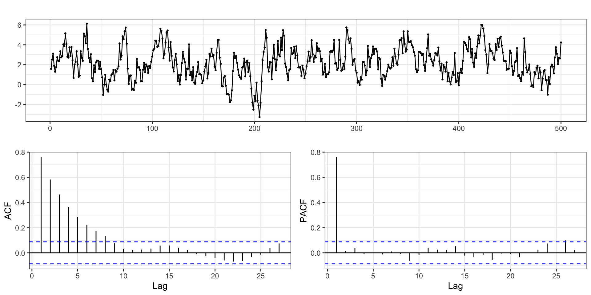
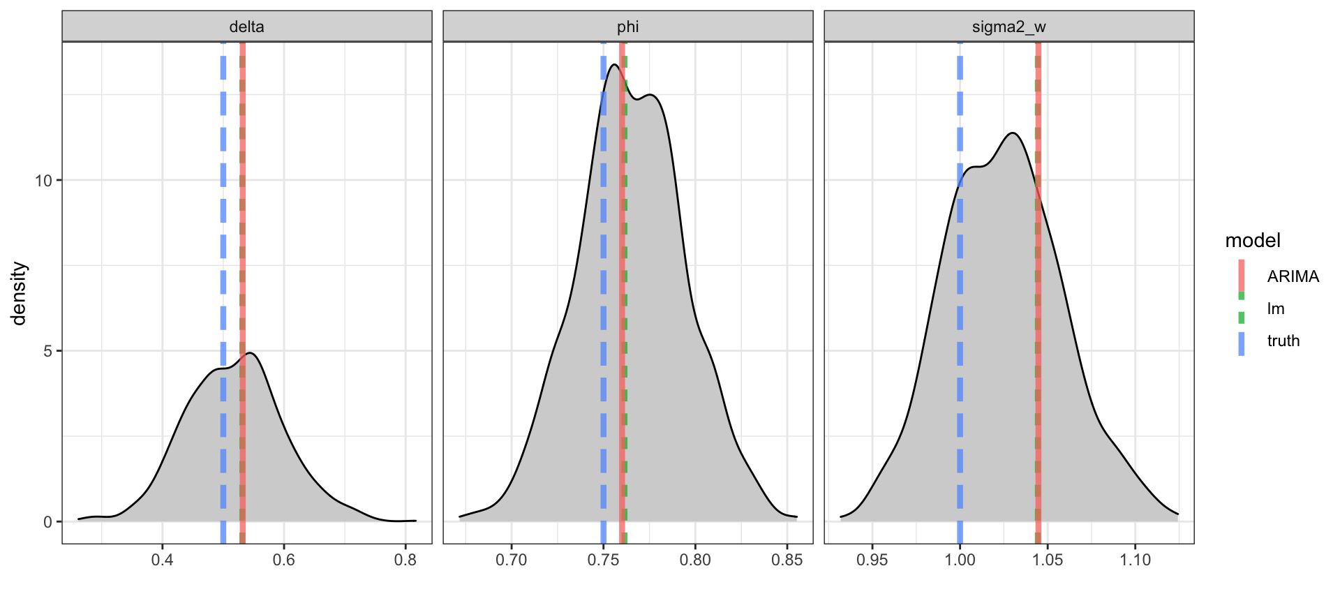
with \(\phi = 0.75\), \(\delta=0.5\), and \(\sigma_w^2=1\),
ARIMA
mean vs \(\delta\)?
The reported mean value from the ARIMA model is \(E(y_t)\) and not \(\delta\) - for an ARIMA(1,0,0) \[ E(y_t) = \frac{\delta}{1-\phi} ~~\Rightarrow~~ \delta = E(y_t) * (1-\phi) \]
lm
d = tsibble::as_tsibble(ar1) %>%
  as_tibble() %>%
  rename(y = value)
summary({ ar1_lm = lm(y~lag(y), data=d) })
Call:
lm(formula = y ~ lag(y), data = d)

Residuals:
    Min      1Q  Median      3Q     Max
-2.7194 -0.6991 -0.0139  0.6323  3.3518

Coefficients:
            Estimate Std. Error t value Pr(>|t|)
(Intercept)  0.53138    0.07898   6.728 4.74e-11 ***
lag(y)       0.76141    0.02918  26.090  < 2e-16 ***
---
Signif. codes:  0 '***' 0.001 '**' 0.01 '*' 0.05 '.' 0.1 ' ' 1

Residual standard error: 1.023 on 497 degrees of freedom
  (1 observation deleted due to missingness)
Multiple R-squared:  0.578, Adjusted R-squared:  0.5771
F-statistic: 680.7 on 1 and 497 DF,  p-value: < 2.2e-16
Bayesian AR(1) Model
library(brms) # must be loaded for arma to work
( ar1_brms = brm(y ~ arma(p = 1, q = 0), data=d, refresh=0) )
Family: gaussian
Links: mu = identity; sigma = identity
Formula: y ~ arma(p = 1, q = 0)
Data: d (Number of observations: 500)
Draws: 4 chains, each with iter = 2000; warmup = 1000; thin = 1;
total post-warmup draws = 4000
Correlation Structures:
Estimate Est.Error l-95% CI u-95% CI Rhat Bulk_ESS Tail_ESS
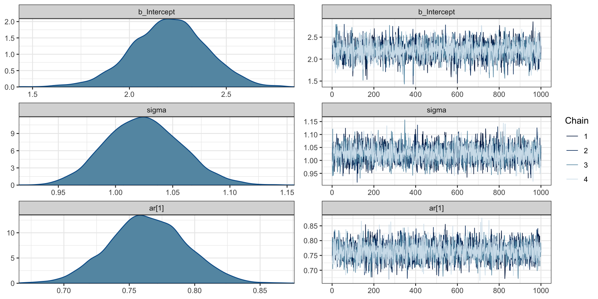
ar[1] 0.76 0.03 0.71 0.82 1.00 3820 2893
Population-Level Effects:
Estimate Est.Error l-95% CI u-95% CI Rhat Bulk_ESS Tail_ESS
Intercept 2.20 0.19 1.82 2.58 1.00 3728 2811
Family Specific Parameters:
Estimate Est.Error l-95% CI u-95% CI Rhat Bulk_ESS Tail_ESS
sigma 1.02 0.03 0.96 1.09 1.00 3889 2940
Draws were sampled using sampling(NUTS). For each parameter, Bulk_ESS
and Tail_ESS are effective sample size measures, and Rhat is the potential
scale reduction factor on split chains (at convergence, Rhat = 1).Chains
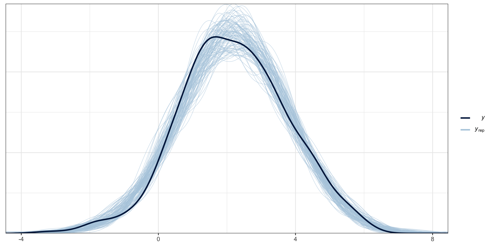
PP Checks
Posteriors
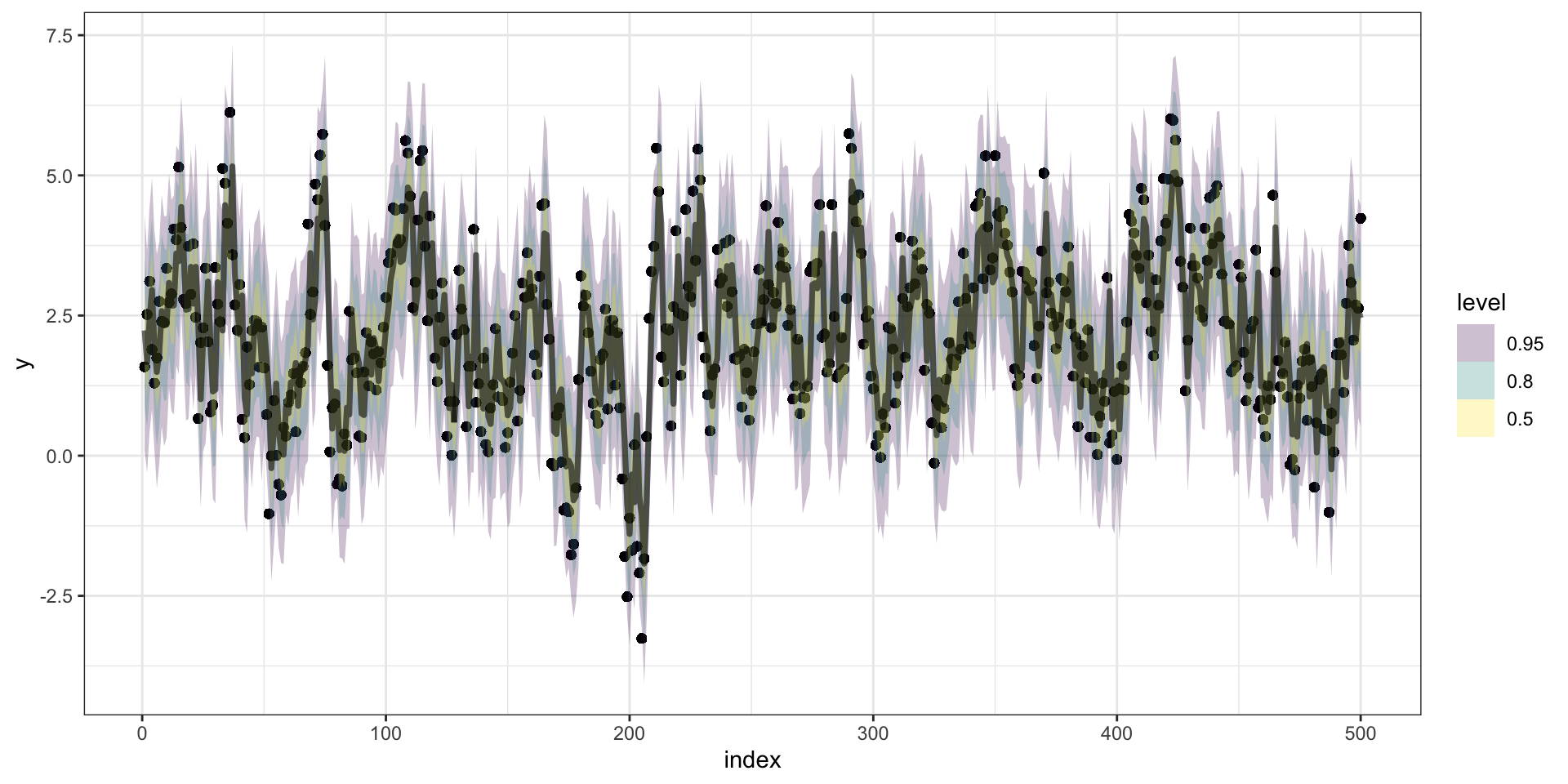
Predictions
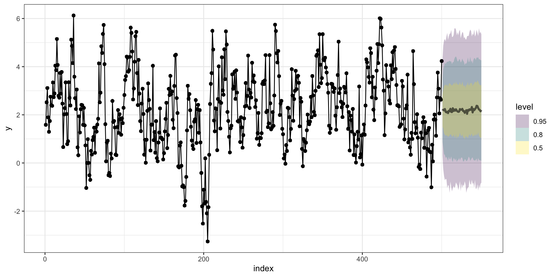
Forecasting
:::
Fitting AR(p)
Lagged Regression
As with the AR(1), we can rewrite the density using conditioning, \[ \begin{aligned} f(\boldsymbol y) &= f(y_t, \,y_{t-1}, \,\ldots, \,y_{2}, \,y_{1}) \\ &= f(y_{n}|y_{n-1},\ldots,y_{n-p}) \cdots f(y_{p+1}|y_p,\ldots,y_1) f(y_p, \,\ldots, y_1) \end{aligned} \]
Regressing \(y_t\) on \(y_{t-1}, \ldots, y_{t-p}\) gets us an approximate solution, but it ignores the \(f(y_1, \, y_2, \,\ldots, y_p)\) part of the likelihood.
How much does this matter (vs. using the full likelihood)?
If \(p\) is near to \(n\) then probably a lot
If \(p << n\) then probably not much
Method of Moments
Recall for an AR(p) process,
\[ \begin{aligned} \gamma(0) &= \sigma^2_w + \phi_1 \gamma(1) + \phi_2 \gamma(2) + \ldots + \phi_p \gamma(p) \\ \gamma(h) &= \phi_1 \gamma(h-1) + \phi_2 \gamma(h-2) + \ldots \phi_p \gamma(h-p) \end{aligned} \] We can rewrite the first equation in terms of \(\sigma^2_w\), \[ \sigma^2_w = \gamma(0) - \phi_1 \gamma(1) - \phi_2 \gamma(2) - \ldots - \phi_p \gamma(p) \] these are called the Yule-Walker equations.
Yule-Walker
These equations can be rewritten into matrix notation as follows
\[ \underset{p \times p}{\boldsymbol\Gamma_p} \underset{p \times 1}{\boldsymbol\phi} = \underset{p \times 1}{\boldsymbol\gamma_p} \qquad\qquad \underset{1 \times 1}{\sigma^2_w} = \underset{1 \times 1}{\gamma(0)} - \underset{1 \times p}{\boldsymbol{\phi'}}\underset{p \times 1}{\boldsymbol{\gamma_p}} \] where
\[ \begin{aligned} \underset{p \times p}{\boldsymbol{\Gamma_p}} &= \{\gamma(j-k)\}_{j,k} \\ \underset{p \times 1}{\boldsymbol\phi} &= (\phi_1, \phi_2, \ldots, \phi_p)' \\ \underset{p \times 1}{\boldsymbol\gamma_p} &= (\gamma(1), \gamma(2), \ldots, \gamma(p))' \end{aligned} \]
If we estimate the covariance structure from the data we obtain \(\hat{\boldsymbol\gamma_p}\) and \(\hat{\boldsymbol\Gamma_p}\) which we can plug in and solve for \(\boldsymbol{\phi}\) and \(\sigma^2_w\), \[ \hat{\boldsymbol\phi} =\hat{\boldsymbol{\Gamma}_p}^{-1}\hat{\boldsymbol{\gamma}_p} \qquad\qquad \hat{\sigma}^2_w = \gamma(0) - \hat{\boldsymbol{\gamma}_p}' \hat{\boldsymbol{\Gamma}_p^{-1}} \hat{\boldsymbol{\gamma}_p} \]
ARMA
Fitting \(ARMA(2,2)\)
\[ y_t = \delta + \phi_1 \, y_{t-1} + \phi_2 \, y_{t-2} + \theta_1 w_{t-1} + \theta_2 w_{t-2} + w_t \]
We now need to estimate six parameters: \(\delta\), \(\phi_1\), \(\phi_2\), \(\theta_1\), \(\theta_2\) and \(\sigma_w^2\).
\(~\)
We could figure out \(E(y_t)\), \(Var(y_t)\), and \(Cov(y_t, y_{t+h})\), but the last two are going to be pretty nasty and the full MVN likehood is similarly going to be unpleasant to work with.
\(~\)
Like the AR(1) and AR(p) processes we want to use conditioning to simplify things. \[ \begin{aligned} y_t | \delta, &y_{t-1}, y_{t-2}, w_{t-1}, w_{t-2} \\ &\sim \mathcal{N}(\delta + \phi_1 \, y_{t-1} + \phi_2 \, y_{t-2} + \theta_1 w_{t-1} + \theta_2 w_{t-2},~\sigma_w^2) \end{aligned} \]
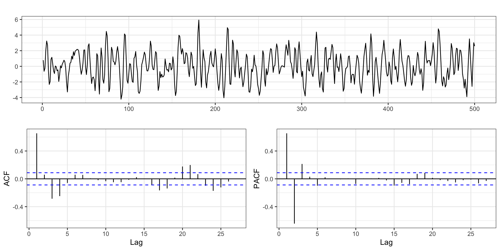
ARMA(2,2) Example
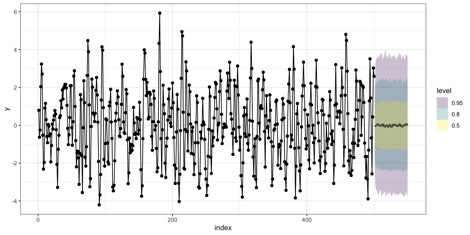
with \(\phi = (0.75,-0.5)\), \(\theta = (0.5,0.2)\), \(\delta=0\), and \(\sigma_w^2=1\) using the same models
ARIMA
Series: y
ARIMA(2,0,2) with zero mean

Coefficients:
         ar1      ar2     ma1     ma2
      0.7290  -0.4967  0.4896  0.2543
s.e.  0.0868   0.0586  0.0940  0.0727

sigma^2 = 1.082:  log likelihood = -728.13
AIC=1466.26   AICc=1466.38   BIC=1487.33

Training set error measures:
                     ME     RMSE       MAE       MPE     MAPE      MASE
Training set 0.02160055 1.036121 0.8309352 -7.423015 270.5659 0.6674512
                     ACF1
Training set -0.001909506
AR only lm
Call:
lm(formula = y ~ lag(y, 1) + lag(y, 2))

Residuals:
     Min       1Q   Median       3Q      Max
-2.95562 -0.69955  0.00587  0.77063  3.13283

Coefficients:
            Estimate Std. Error t value Pr(>|t|)
(Intercept)  0.02892    0.04802   0.602    0.547
lag(y, 1)    1.07883    0.03430  31.455   <2e-16 ***
lag(y, 2)   -0.64708    0.03438 -18.820   <2e-16 ***
---
Signif. codes:  0 '***' 0.001 '**' 0.01 '*' 0.05 '.' 0.1 ' ' 1

Residual standard error: 1.071 on 495 degrees of freedom
  (2 observations deleted due to missingness)
Multiple R-squared:  0.6677,    Adjusted R-squared:  0.6664
F-statistic: 497.4 on 2 and 495 DF,  p-value: < 2.2e-16
Hannan-Rissanen Algorithm
Estimate a high order AR (remember AR \(\Leftrightarrow\) MA when stationary + invertible)
Use AR to estimate values for unobserved \(w_t\) via
lmwithlagsRegress \(y_t\) onto \(y_{t-1}, \ldots, y_{t-p}, \hat{w}_{t-1}, \ldots \hat{w}_{t-q}\)
Update \(\hat{w}_{t-1}, \ldots \hat{w}_{t-q}\) based on current model,
Goto 3, repeat until convergence
Hannan-Rissanen - Step 1 & 2
Series: y
ARIMA(10,0,0) with non-zero mean

Coefficients:
         ar1      ar2     ar3     ar4      ar5
      1.2162  -0.8378  0.0927  0.1693  -0.1274
s.e.  0.0446   0.0702  0.0796  0.0800   0.0807
         ar6     ar7      ar8     ar9     ar10
      0.0198  0.0274  -0.0841  0.1001  -0.0736
s.e.  0.0809  0.0809   0.0808  0.0713   0.0453
        mean
      0.0501
s.e.  0.0930

sigma^2 = 1.09:  log likelihood = -726.47
AIC=1476.93   AICc=1477.57   BIC=1527.51
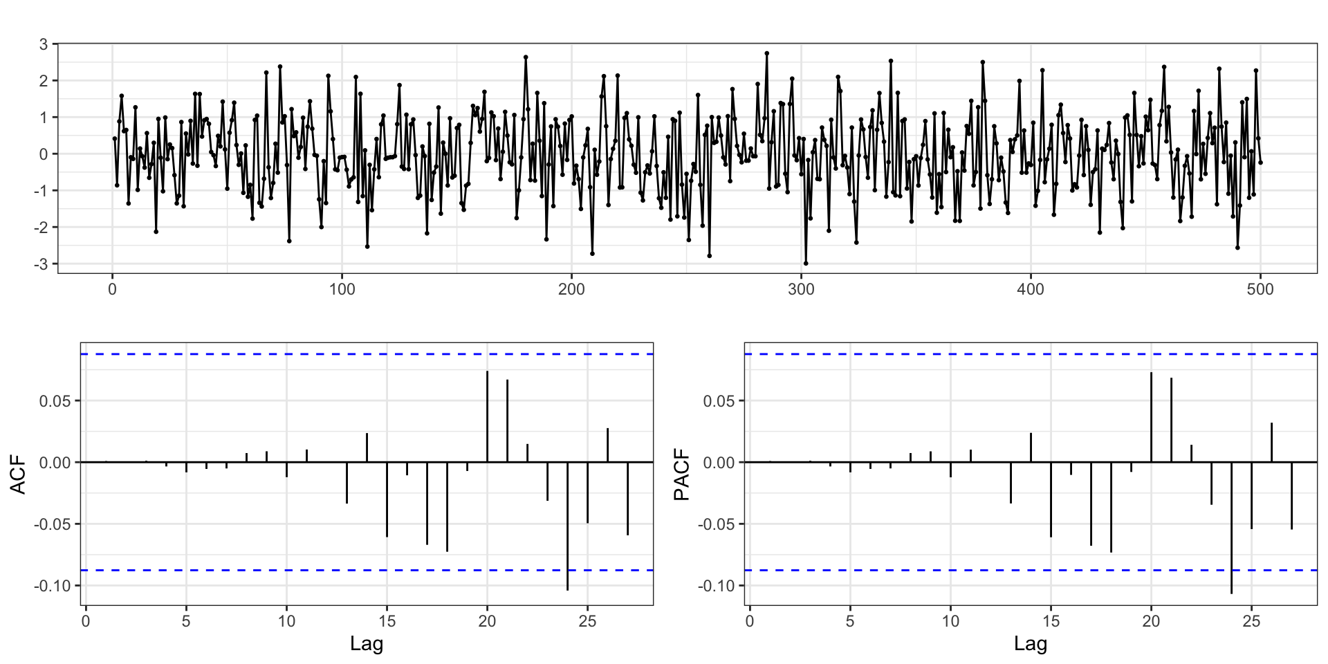
Residuals
Hannan-Rissanen - Step 3
d = tibble(
  y = y %>% strip_attr(),
  index = seq_along(y),
  w_hat1 = ar$resid %>% strip_attr()
)

(lm1 = lm(y ~ lag(y,1) + lag(y,2) + lag(w_hat1,1) + lag(w_hat1,2), data=d)) %>%
  summary()
Call:
lm(formula = y ~ lag(y, 1) + lag(y, 2) + lag(w_hat1, 1) + lag(w_hat1,
    2), data = d)

Residuals:
     Min       1Q   Median       3Q      Max
-2.95099 -0.67750 -0.06171  0.71850  2.76012

Coefficients:
               Estimate Std. Error t value Pr(>|t|)
(Intercept)     0.03851    0.04682   0.822  0.41120
lag(y, 1)       0.75235    0.07460  10.085  < 2e-16 ***
lag(y, 2)      -0.50700    0.04260 -11.901  < 2e-16 ***
lag(w_hat1, 1)  0.46543    0.08735   5.328 1.51e-07 ***
lag(w_hat1, 2)  0.23369    0.08193   2.852  0.00452 **
---
Signif. codes:  0 '***' 0.001 '**' 0.01 '*' 0.05 '.' 0.1 ' ' 1

Residual standard error: 1.043 on 493 degrees of freedom
  (2 observations deleted due to missingness)
Multiple R-squared:  0.6861,    Adjusted R-squared:  0.6836
F-statistic: 269.4 on 4 and 493 DF,  p-value: < 2.2e-16
Hannan-Rissanen - Step 4
d = modelr::add_residuals(d,lm1,"w_hat2")

(lm2 = lm(y ~ lag(y,1) + lag(y,2) + lag(w_hat2,1) + lag(w_hat2,2), data=d)) %>%
  summary()
Call:
lm(formula = y ~ lag(y, 1) + lag(y, 2) + lag(w_hat2, 1) + lag(w_hat2,
    2), data = d)

Residuals:
     Min       1Q   Median       3Q      Max
-2.94460 -0.66888 -0.05112  0.74813  2.82163

Coefficients:
               Estimate Std. Error t value Pr(>|t|)
(Intercept)     0.03373    0.04685   0.720  0.47187
lag(y, 1)       0.75142    0.07501  10.017  < 2e-16 ***
lag(y, 2)      -0.50683    0.04271 -11.866  < 2e-16 ***
lag(w_hat2, 1)  0.46357    0.08737   5.306  1.7e-07 ***
lag(w_hat2, 2)  0.23568    0.08183   2.880  0.00415 **
---
Signif. codes:  0 '***' 0.001 '**' 0.01 '*' 0.05 '.' 0.1 ' ' 1

Residual standard error: 1.042 on 491 degrees of freedom
  (4 observations deleted due to missingness)
Multiple R-squared:  0.6877,    Adjusted R-squared:  0.6851
F-statistic: 270.3 on 4 and 491 DF,  p-value: < 2.2e-16
Hannan-Rissanen - Step 3.2 + 4.2
d = modelr::add_residuals(d,lm2,"w_hat3")

(lm3 = lm(y ~ lag(y,1) + lag(y,2) + lag(w_hat3,1) + lag(w_hat3,2), data=d)) %>%
  summary()
Call:
lm(formula = y ~ lag(y, 1) + lag(y, 2) + lag(w_hat3, 1) + lag(w_hat3,
    2), data = d)

Residuals:
     Min       1Q   Median       3Q      Max
-2.97513 -0.67010 -0.04563  0.76228  2.78317

Coefficients:
               Estimate Std. Error t value Pr(>|t|)
(Intercept)     0.02734    0.04700   0.582  0.56097
lag(y, 1)       0.75611    0.07540  10.028  < 2e-16 ***
lag(y, 2)      -0.50692    0.04287 -11.826  < 2e-16 ***
lag(w_hat3, 1)  0.45652    0.08791   5.193 3.05e-07 ***
lag(w_hat3, 2)  0.22498    0.08228   2.734  0.00648 **
---
Signif. codes:  0 '***' 0.001 '**' 0.01 '*' 0.05 '.' 0.1 ' ' 1

Residual standard error: 1.044 on 489 degrees of freedom
  (6 observations deleted due to missingness)
Multiple R-squared:  0.6845,    Adjusted R-squared:  0.6819
F-statistic: 265.2 on 4 and 489 DF,  p-value: < 2.2e-16
Hannan-Rissanen - Step 3.3 + 4.3
d = modelr::add_residuals(d,lm3,"w_hat4")

(lm4 = lm(y ~ lag(y,1) + lag(y,2) + lag(w_hat4,1) + lag(w_hat4,2), data=d)) %>%
  summary()
Call:
lm(formula = y ~ lag(y, 1) + lag(y, 2) + lag(w_hat4, 1) + lag(w_hat4,
    2), data = d)

Residuals:
     Min       1Q   Median       3Q      Max
-2.95836 -0.66815 -0.03775  0.74089  2.77938

Coefficients:
               Estimate Std. Error t value Pr(>|t|)
(Intercept)     0.02909    0.04699   0.619  0.53614
lag(y, 1)       0.73928    0.07567   9.769  < 2e-16 ***
lag(y, 2)      -0.50025    0.04291 -11.657  < 2e-16 ***
lag(w_hat4, 1)  0.47626    0.08791   5.417 9.52e-08 ***
lag(w_hat4, 2)  0.24343    0.08248   2.951  0.00332 **
---
Signif. codes:  0 '***' 0.001 '**' 0.01 '*' 0.05 '.' 0.1 ' ' 1

Residual standard error: 1.042 on 487 degrees of freedom
  (8 observations deleted due to missingness)
Multiple R-squared:  0.6859,    Adjusted R-squared:  0.6833
F-statistic: 265.8 on 4 and 487 DF,  p-value: < 2.2e-16
Hannan-Rissanen - Step 3.4 + 4.4
d = modelr::add_residuals(d,lm4,"w_hat5")

(lm5 = lm(y ~ lag(y,1) + lag(y,2) + lag(w_hat5,1) + lag(w_hat5,2), data=d)) %>%
  summary()
Call:
lm(formula = y ~ lag(y, 1) + lag(y, 2) + lag(w_hat5, 1) + lag(w_hat5,
    2), data = d)

Residuals:
     Min       1Q   Median       3Q      Max
-2.96227 -0.68428 -0.04699  0.75613  2.77697

Coefficients:
               Estimate Std. Error t value Pr(>|t|)
(Intercept)     0.02844    0.04721   0.602  0.54724
lag(y, 1)       0.75159    0.07681   9.785  < 2e-16 ***
lag(y, 2)      -0.50072    0.04335 -11.551  < 2e-16 ***
lag(w_hat5, 1)  0.46345    0.08938   5.185 3.18e-07 ***
lag(w_hat5, 2)  0.22949    0.08355   2.747  0.00624 **
---
Signif. codes:  0 '***' 0.001 '**' 0.01 '*' 0.05 '.' 0.1 ' ' 1

Residual standard error: 1.044 on 485 degrees of freedom
  (10 observations deleted due to missingness)
Multiple R-squared:  0.685, Adjusted R-squared:  0.6824
F-statistic: 263.6 on 4 and 485 DF,  p-value: < 2.2e-16
BRMS
 Family: gaussian
  Links: mu = identity; sigma = identity
Formula: y ~ arma(p = 2, q = 2) - 1
   Data: d (Number of observations: 500)
  Draws: 2 chains, each with iter = 5000; warmup = 2500; thin = 1;
         total post-warmup draws = 5000

Correlation Structures:
      Estimate Est.Error l-95% CI u-95% CI Rhat Bulk_ESS Tail_ESS
ar[1]     0.73      0.09     0.54     0.90 1.00      789      967
ar[2]    -0.49      0.06    -0.60    -0.36 1.00     1237     1288
ma[1]     0.49      0.10     0.29     0.68 1.00      795     1054
ma[2]     0.25      0.08     0.09     0.39 1.00      873     1280

Family Specific Parameters:
      Estimate Est.Error l-95% CI u-95% CI Rhat Bulk_ESS Tail_ESS
sigma     1.05      0.03     0.98     1.11 1.00     6406     3711

Draws were sampled using sampling(NUTS). For each parameter, Bulk_ESS
and Tail_ESS are effective sample size measures, and Rhat is the potential
scale reduction factor on split chains (at convergence, Rhat = 1).
Chains
Comparison

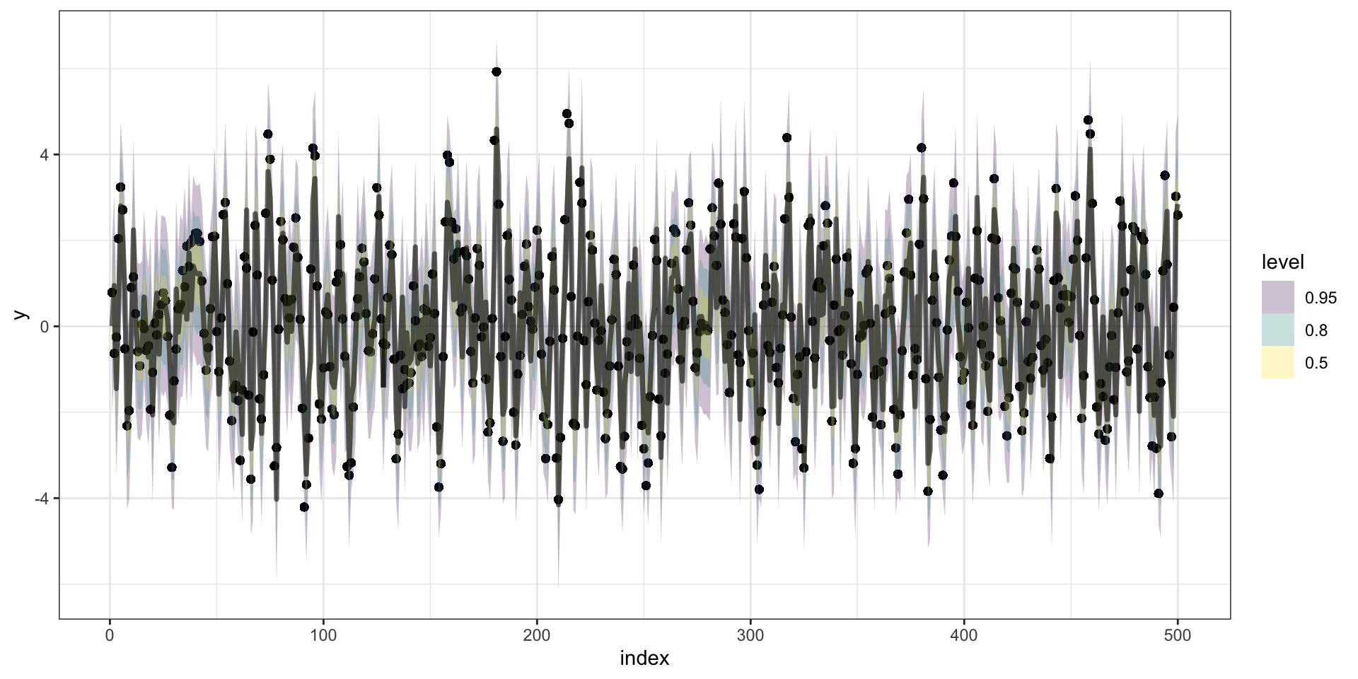
Predictions
Forecasting
Stan Code
// generated with brms 2.18.0
functions {
}
data {
  int<lower=1> N;  // total number of observations
  vector[N] Y;  // response variable
  // data needed for ARMA correlations
  int<lower=0> Kar;  // AR order
  int<lower=0> Kma;  // MA order
  // number of lags per observation
  int<lower=0> J_lag[N];
  int prior_only;  // should the likelihood be ignored?
}
transformed data {
  int max_lag = max(Kar, Kma);
}
parameters {
  vector[Kar] ar;  // autoregressive coefficients
  vector[Kma] ma;  // moving-average coefficients
  real<lower=0> sigma;  // dispersion parameter
}
transformed parameters {
  real lprior = 0;  // prior contributions to the log posterior
  lprior += student_t_lpdf(sigma | 3, 0, 2.5)
    - 1 * student_t_lccdf(0 | 3, 0, 2.5);
}
model {
  // likelihood including constants
  if (!prior_only) {
    // matrix storing lagged residuals
    matrix[N, max_lag] Err = rep_matrix(0, N, max_lag);
    vector[N] err;  // actual residuals
    // initialize linear predictor term
    vector[N] mu = rep_vector(0.0, N);
    // include ARMA terms
    for (n in 1:N) {
      mu[n] += Err[n, 1:Kma] * ma;
      err[n] = Y[n] - mu[n];
      for (i in 1:J_lag[n]) {
        Err[n + 1, i] = err[n + 1 - i];
      }
      mu[n] += Err[n, 1:Kar] * ar;
    }
    target += normal_lpdf(Y | mu, sigma);
  }
  // priors including constants
  target += lprior;
}
generated quantities {
}
Sta 344 - Fall 2022
