Seasonal Arima

Lecture 11

Dr. Colin Rundel

ARIMA - General Guidance

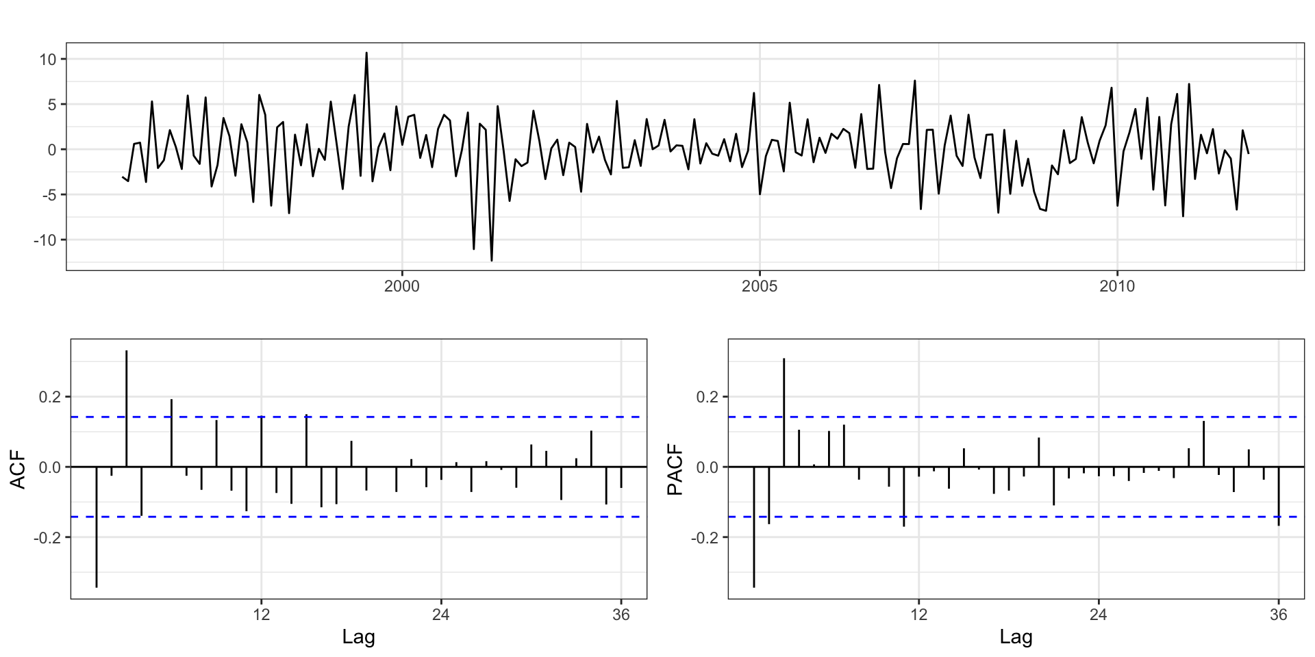
  1. Positive autocorrelations out to a large number of lags usually indicates a need for differencing

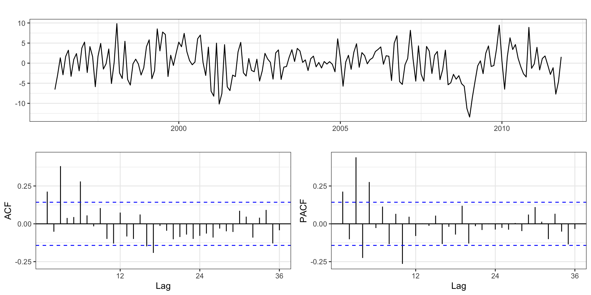
  2. Slightly too much or slightly too little differencing can be corrected by adding AR or MA terms respectively.

  3. A model with no differencing usually includes a constant term, a model with two or more orders (rare) differencing usually does not include a constant term.

  4. After differencing, if the PACF has a sharp cutoff then consider adding AR terms to the model.

  5. After differencing, if the ACF has a sharp cutoff then consider adding an MA term to the model.

  6. It is possible for an AR term and an MA term to cancel each other’s effects, so try models with fewer AR terms and fewer MA terms.

Electrical Equipment Sales

Data
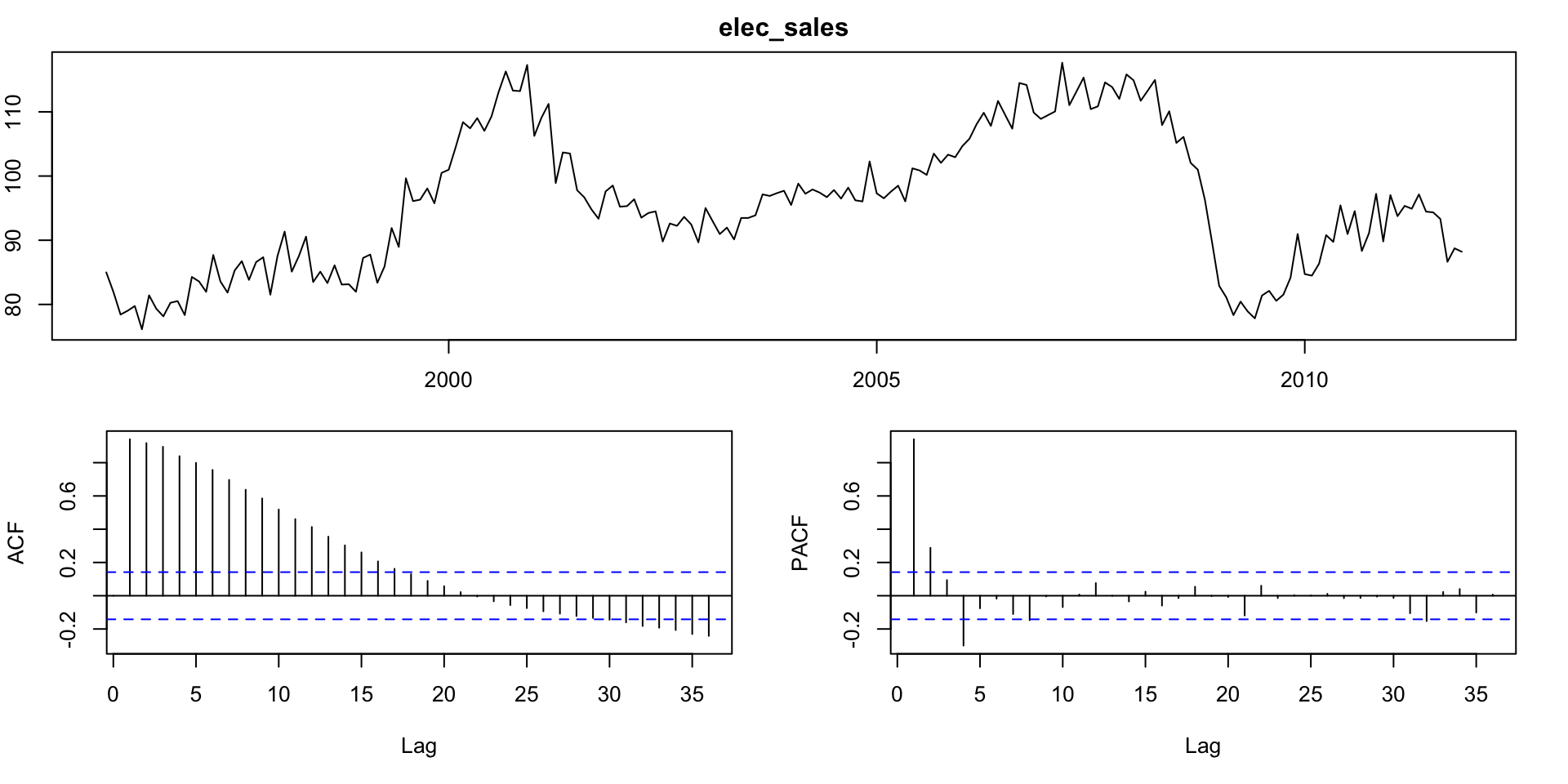
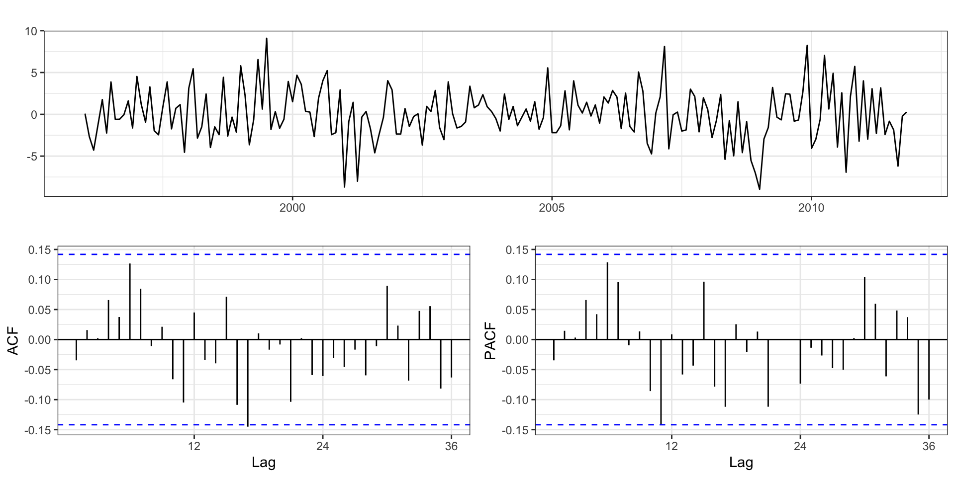
1st order differencing
2nd order differencing
Model

forecast::Arima(elec_sales, order = c(3,1,0))
Series: elec_sales 
ARIMA(3,1,0) 

Coefficients:
          ar1      ar2     ar3
      -0.3488  -0.0386  0.3139
s.e.   0.0690   0.0736  0.0694

sigma^2 = 9.853:  log likelihood = -485.67
AIC=979.33   AICc=979.55   BIC=992.32

Residuals

forecast::Arima(elec_sales, order = c(3,1,0)) %>% residuals() %>% 
  forecast::ggtsdisplay(points=FALSE)

Model Comparison

Model choices:

forecast::Arima(elec_sales, order = c(3,1,0))$aicc
[1] 979.5477
forecast::Arima(elec_sales, order = c(3,1,1))$aicc
[1] 978.4925
forecast::Arima(elec_sales, order = c(4,1,0))$aicc
[1] 979.2309
forecast::Arima(elec_sales, order = c(2,1,0))$aicc
[1] 996.8085

Automatic selection (AICc)

forecast::auto.arima(elec_sales)
Series: elec_sales 
ARIMA(3,1,1) 

Coefficients:
         ar1     ar2     ar3      ma1
      0.0519  0.1191  0.3730  -0.4542
s.e.  0.1840  0.0888  0.0679   0.1993

sigma^2 = 9.737:  log likelihood = -484.08
AIC=978.17   AICc=978.49   BIC=994.4

Automatic selection (BIC)

forecast::auto.arima(elec_sales, ic = "bic")
Series: elec_sales 
ARIMA(1,1,2) 

Coefficients:
         ar1      ma1     ma2
      0.7738  -1.2298  0.5106
s.e.  0.0933   0.1035  0.0695

sigma^2 = 10.2:  log likelihood = -488.99
AIC=985.97   AICc=986.19   BIC=998.96

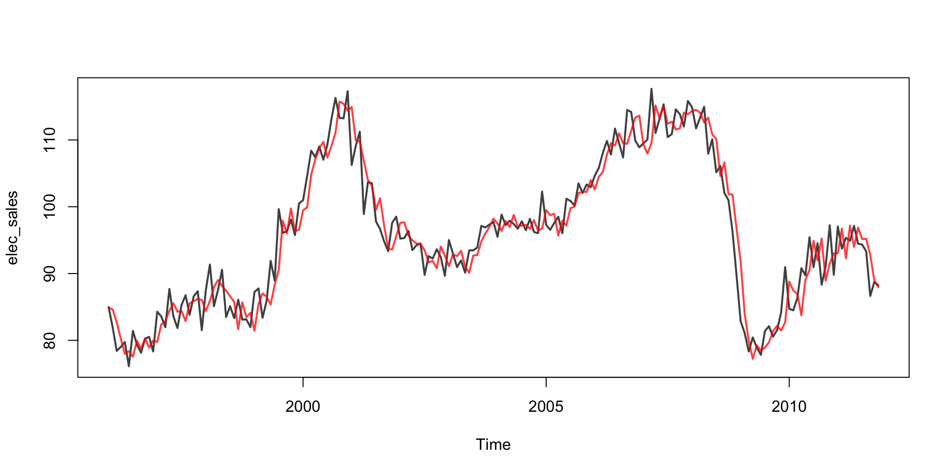
Model fit

plot(elec_sales, lwd=2, col=adjustcolor("black", alpha.f=0.75))
forecast::Arima(elec_sales, order = c(3,1,0)) %>% fitted() %>% 
  lines(col=adjustcolor('red',alpha.f=0.75),lwd=2)

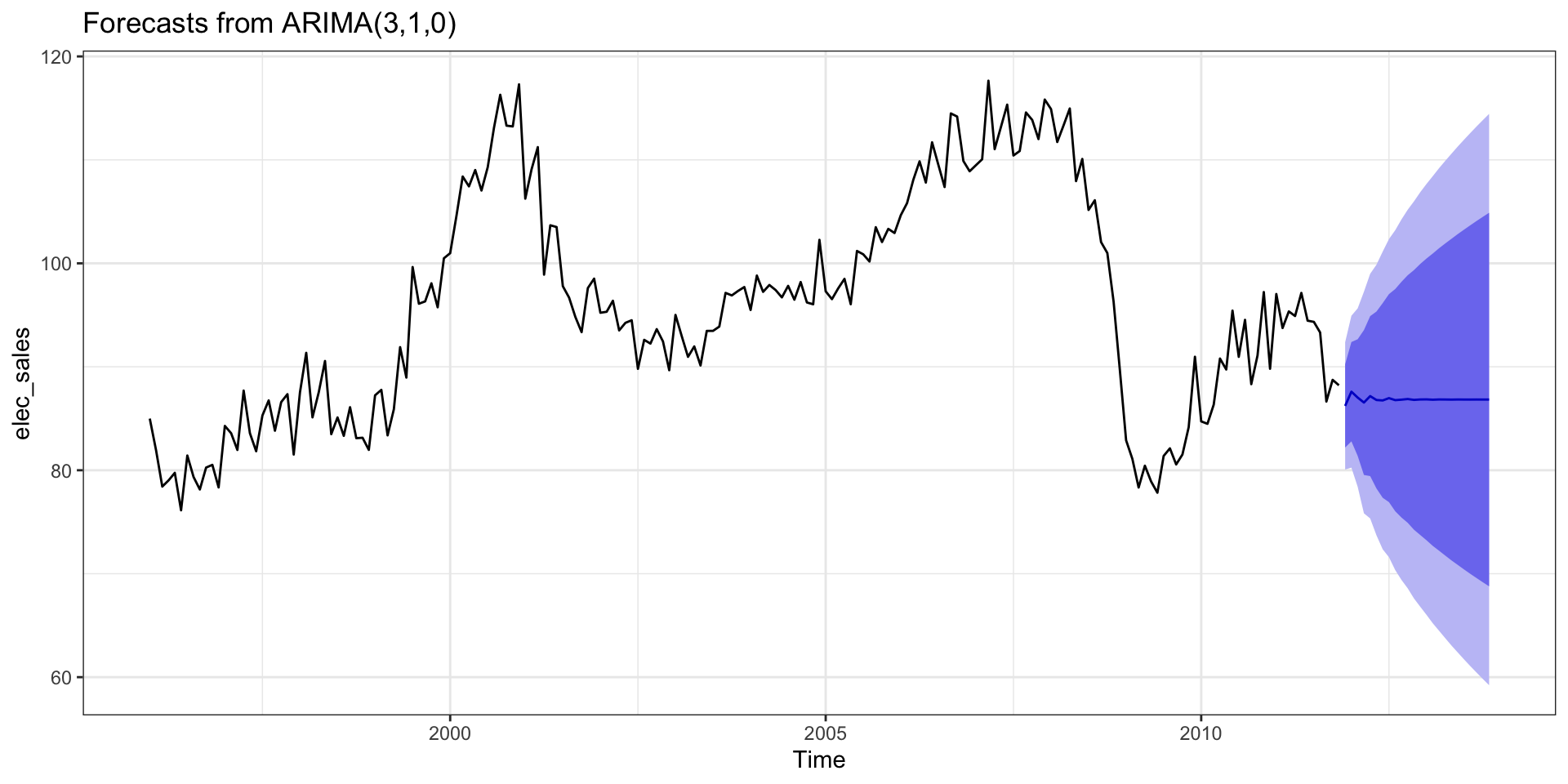
Model forecast

forecast::Arima(elec_sales, order = c(3,1,0)) %>% 
  forecast::forecast() %>% autoplot()

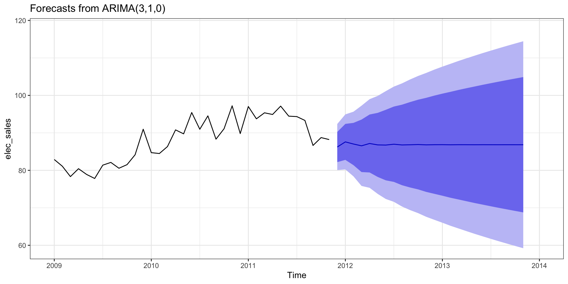
Model forecast - Zoom

forecast::Arima(elec_sales, order = c(3,1,0)) %>% 
  forecast::forecast() %>% autoplot() + xlim(2009,2014)

Seasonal Models

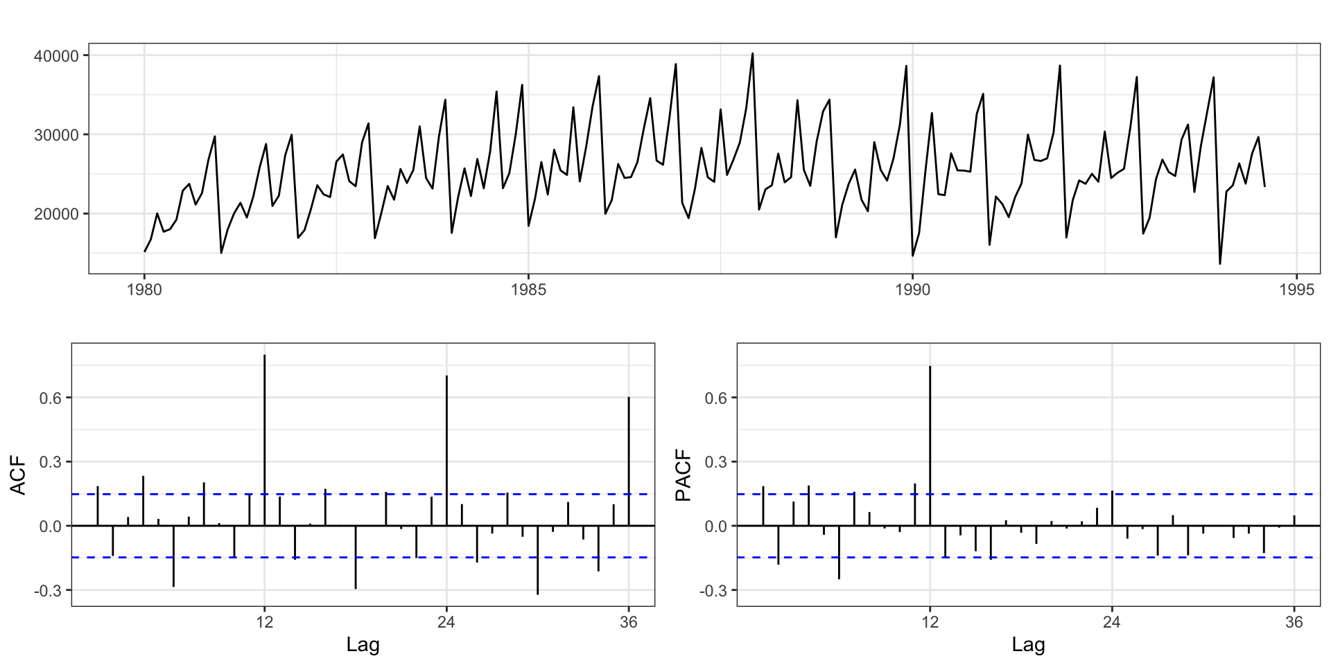
Australian Wine Sales Example

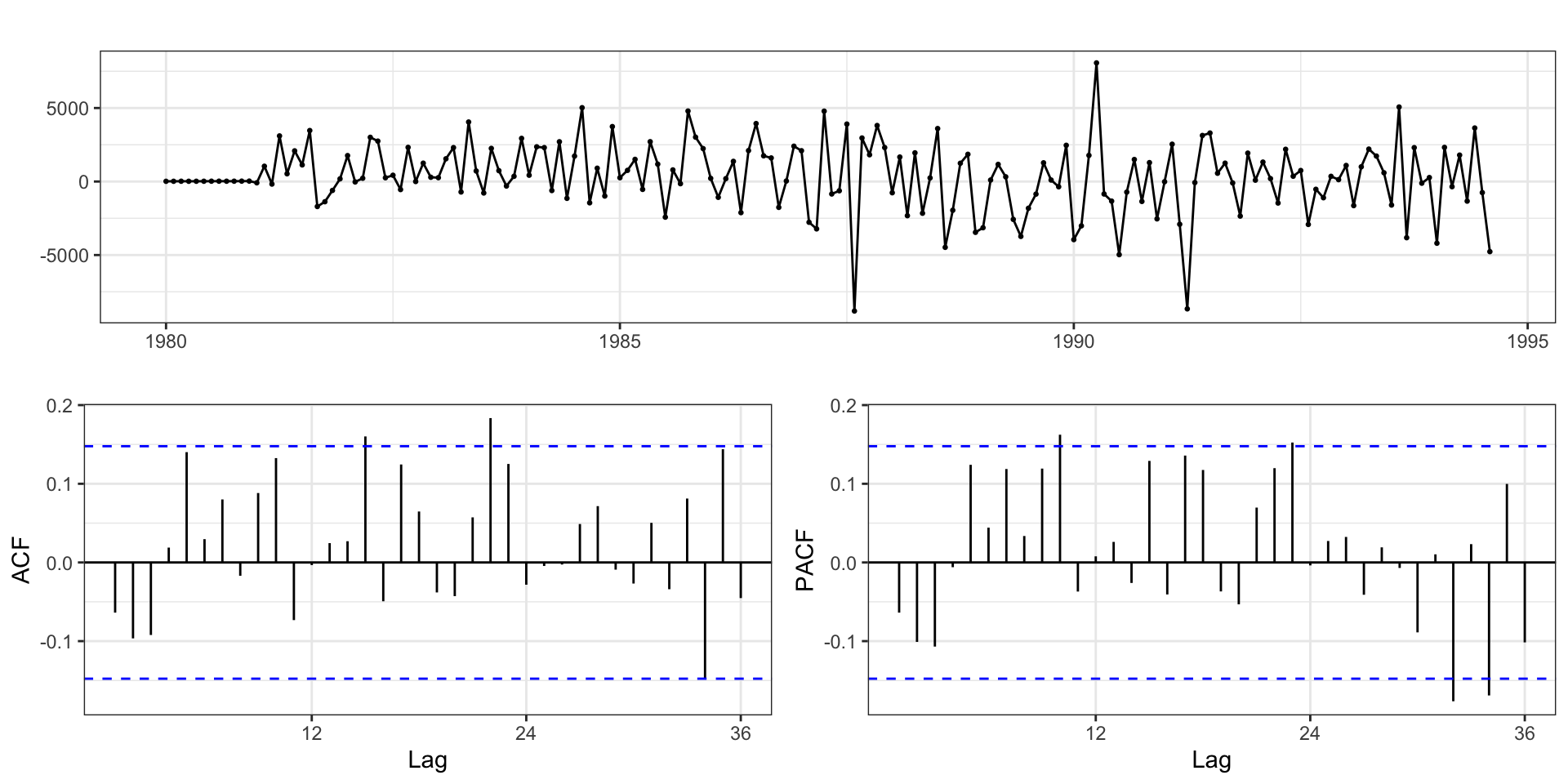
Australian total wine sales by wine makers in bottles <= 1 litre. Jan 1980 – Aug 1994.
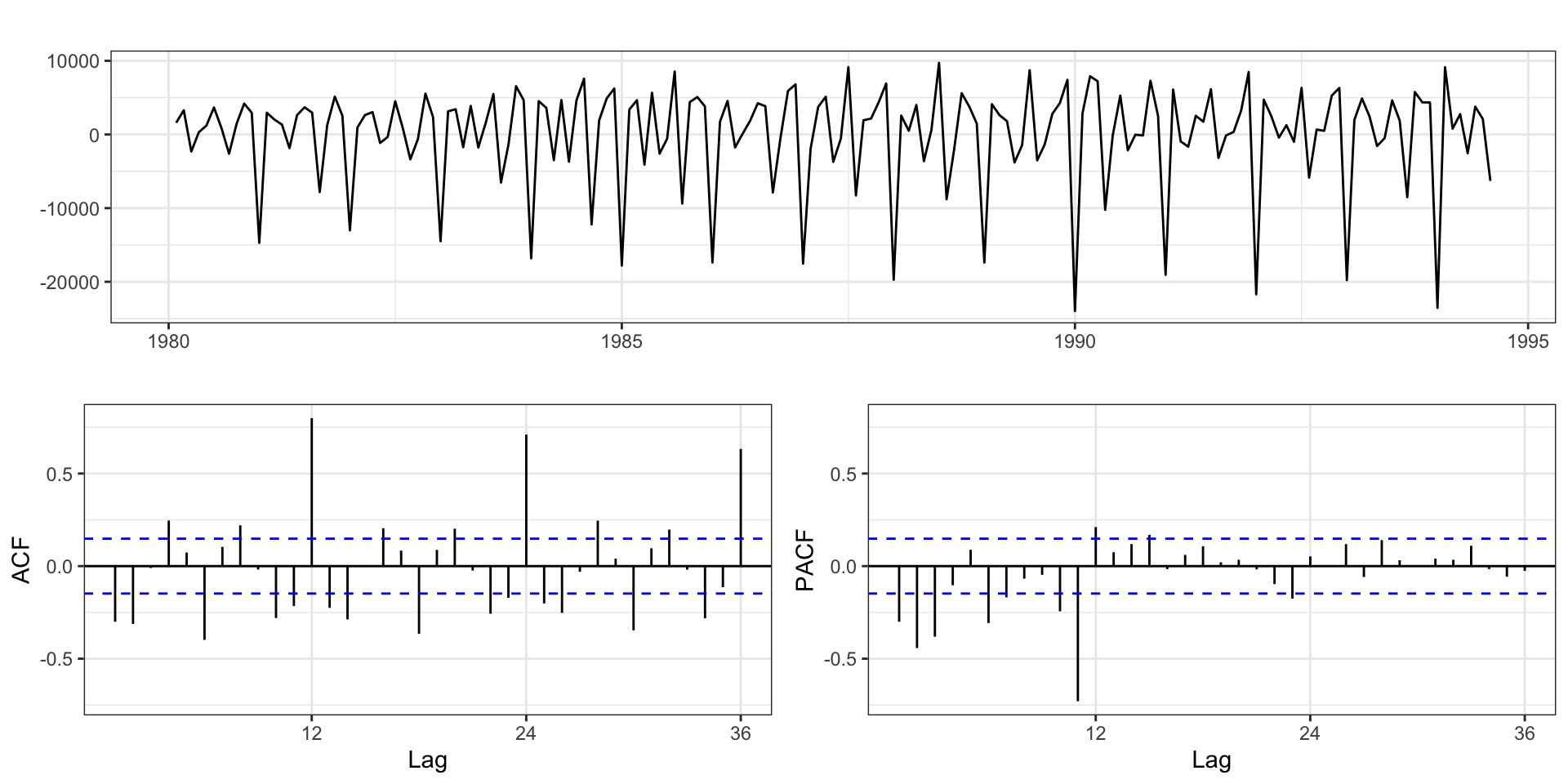
Differencing
Seasonal Arima

We can extend the existing ARIMA model to handle these higher order lags (without having to include all of the intervening lags).

Seasonal \(\text{ARIMA}\,(p,d,q) \times (P,D,Q)_s\): \[ \Phi_P(L^s) \, \phi_p(L) \, \Delta_s^D \, \Delta^d \, y_t = \delta + \Theta_Q(L^s) \, \theta_q(L) \, w_t\] . . .

where

\[ \begin{aligned} \phi_p(L) &= 1-\phi_1 L - \phi_2 L^2 - \ldots - \phi_p L^p\\ \theta_q(L) &= 1+\theta_1 L + \theta_2 L^2 + \ldots + \theta_p L^q \\ \Delta^d &= (1-L)^d\\ \\ \Phi_P(L^s) &= 1-\Phi_1 L^s - \Phi_2 L^{2s} - \ldots - \Phi_P L^{Ps} \\ \Theta_Q(L^s) &= 1+\Theta_1 L + \Theta_2 L^{2s} + \ldots + \theta_p L^{Qs} \\ \Delta_s^D &= (1-L^s)^D\\ \end{aligned} \]

Seasonal ARIMA - AR

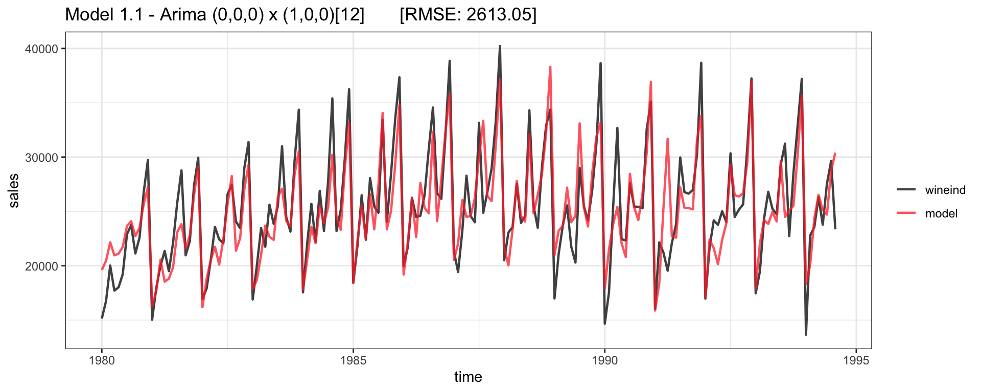
Lets consider an \(\text{ARIMA}(0,0,0) \times (1,0,0)_{12}\): \[ \begin{aligned} (1-\Phi_1 L^{12}) \, y_t = \delta + w_t \\ y_t = \Phi_1 y_{t-12} + \delta + w_t \end{aligned} \]

(m1.1 = forecast::Arima(wineind, seasonal=list(order=c(1,0,0), period=12)))
Series: wineind 
ARIMA(0,0,0)(1,0,0)[12] with non-zero mean 

Coefficients:
        sar1       mean
      0.8780  24489.243
s.e.  0.0314   1154.487

sigma^2 = 6906536:  log likelihood = -1643.39
AIC=3292.78   AICc=3292.92   BIC=3302.29

Fitted - Model 1.1

Seasonal Arima - Diff

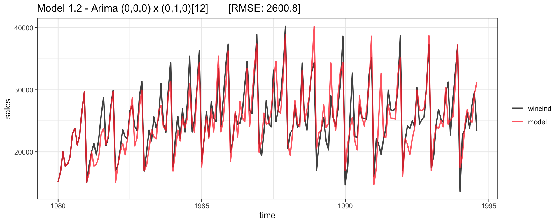
Lets consider an \(\text{ARIMA}(0,0,0) \times (0,1,0)_{12}\): \[ \begin{aligned} (1 - L^{12}) \, y_t = \delta + w_t \\ y_t = y_{t-12} + \delta + w_t \end{aligned} \]

(m1.2 = forecast::Arima(
  wineind, seasonal=list(order=c(0,1,0), period=12)
))
Series: wineind 
ARIMA(0,0,0)(0,1,0)[12] 

sigma^2 = 7259076:  log likelihood = -1528.12
AIC=3058.24   AICc=3058.27   BIC=3061.34

Fitted - Model 1.2

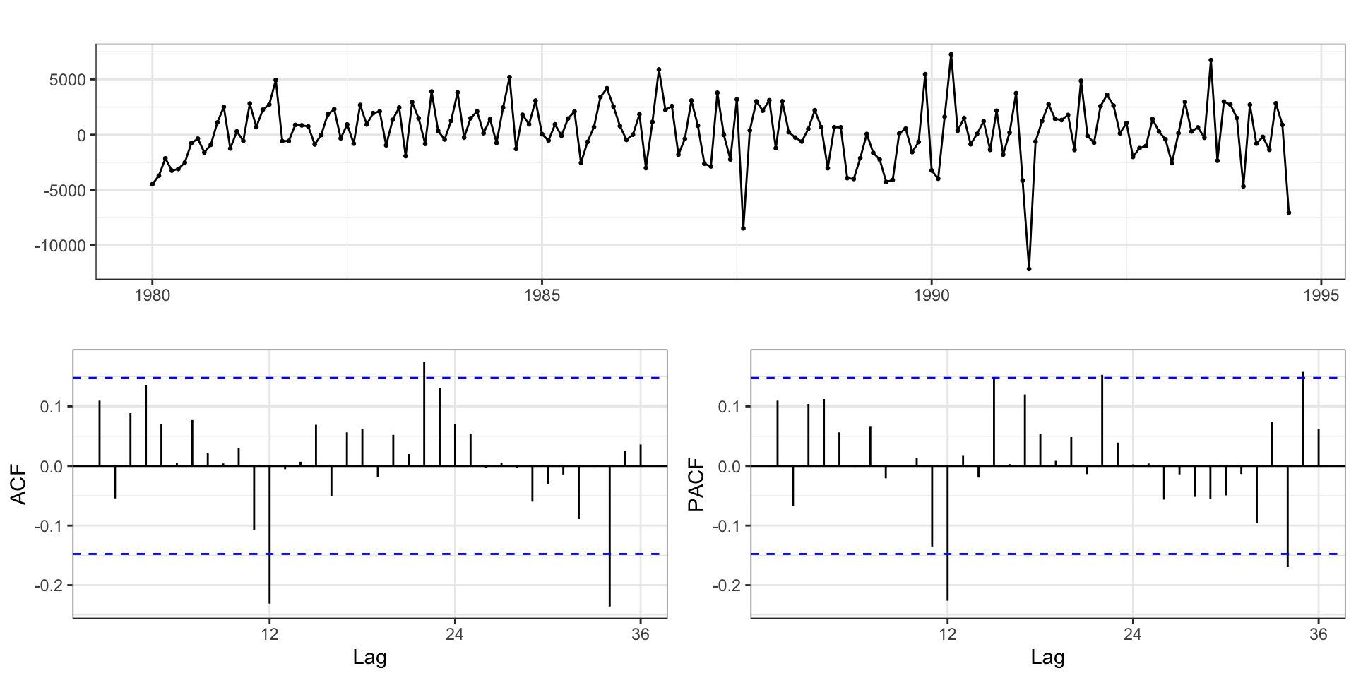
Residuals - Model 1.1 (SAR)
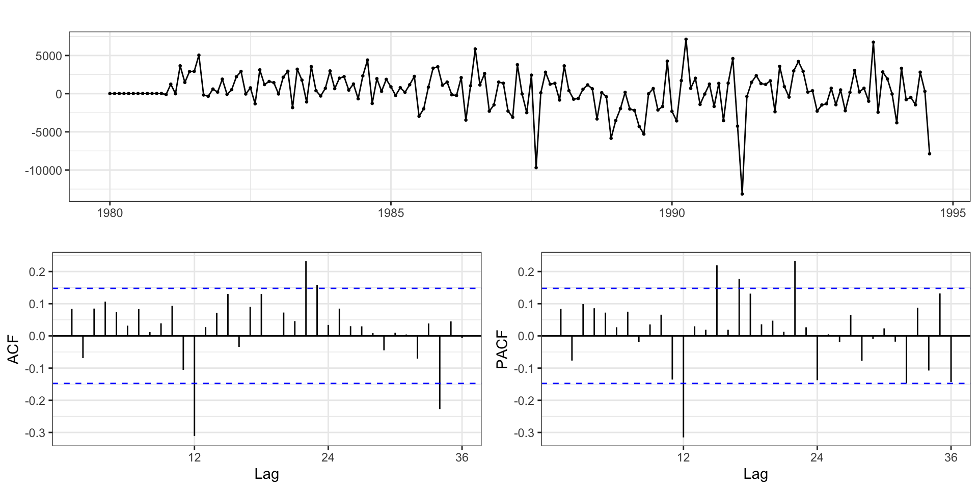
Residuals - Model 1.2 (SDiff)
Model 2

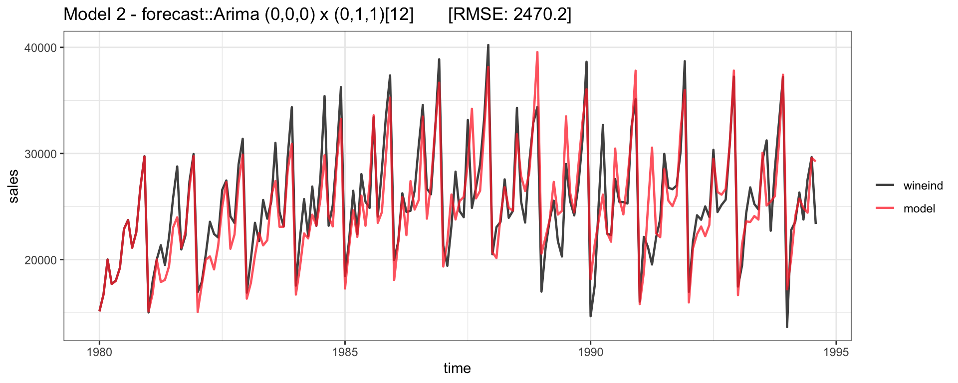
\(\text{ARIMA}(0,0,0) \times (0,1,1)_{12}\):

\[ \begin{aligned} (1-L^{12}) y_t = \delta + (1+\Theta_1 L^{12}) w_t \\ y_t = \delta + y_{t-12} + w_t + \Theta_1 w_{t-12} \end{aligned} \]

(m2 = forecast::Arima(wineind, order=c(0,0,0), 
                      seasonal=list(order=c(0,1,1), period=12)))
Series: wineind 
ARIMA(0,0,0)(0,1,1)[12] 

Coefficients:
         sma1
      -0.3246
s.e.   0.0807

sigma^2 = 6588531:  log likelihood = -1520.34
AIC=3044.68   AICc=3044.76   BIC=3050.88

Fitted - Model 2

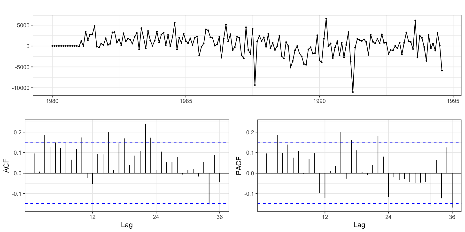
Residuals

Model 3

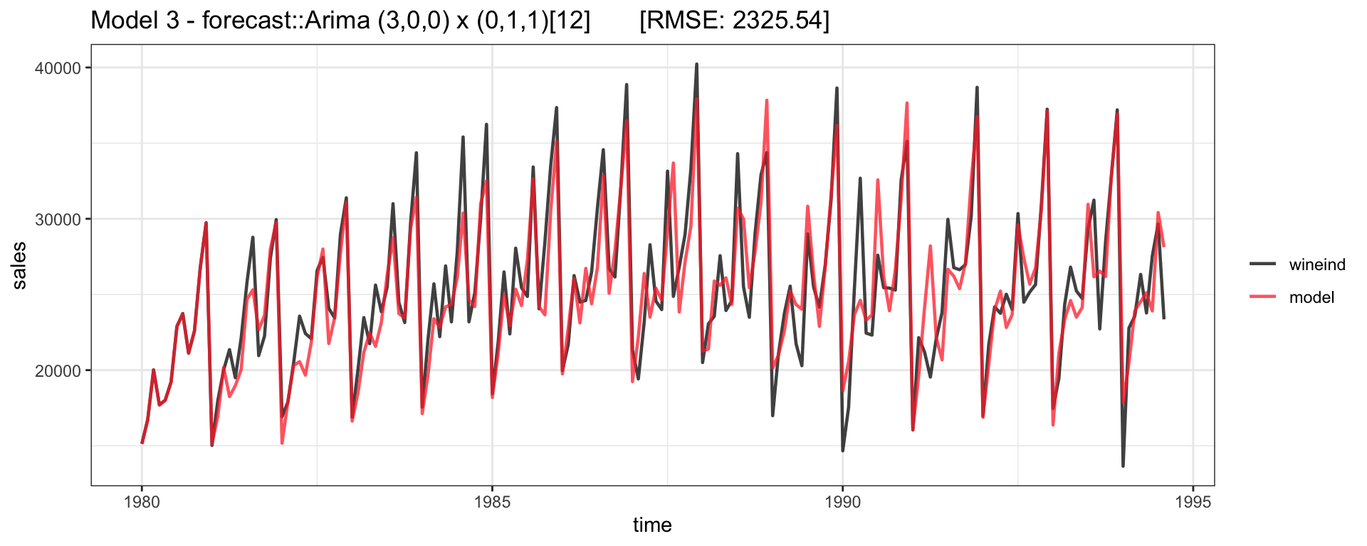
\(\text{ARIMA}(3,0,0) \times (0,1,1)_{12}\)

\[ \begin{aligned} (1-\phi_1 L - \phi_2 L^2 - \phi_3 L^3) \, (1-L^{12}) y_t = \delta + (1 + \Theta_1 L)w_t \\ y_t = \delta + \sum_{i=1}^3 \phi_i y_{t-i} + y_{t-12} - \sum_{i=1}^3 \phi_i y_{t-12-i} + w_t + w_{t-12} \end{aligned} \]

(m3 = forecast::Arima(wineind, order=c(3,0,0), 
                      seasonal=list(order=c(0,1,1), period=12)))
Series: wineind 
ARIMA(3,0,0)(0,1,1)[12] 

Coefficients:
         ar1     ar2     ar3     sma1
      0.1402  0.0806  0.3040  -0.5790
s.e.  0.0755  0.0813  0.0823   0.1023

sigma^2 = 5948935:  log likelihood = -1512.38
AIC=3034.77   AICc=3035.15   BIC=3050.27

Fitted model

Model - Residuals

Federal Reserve Board Production Index

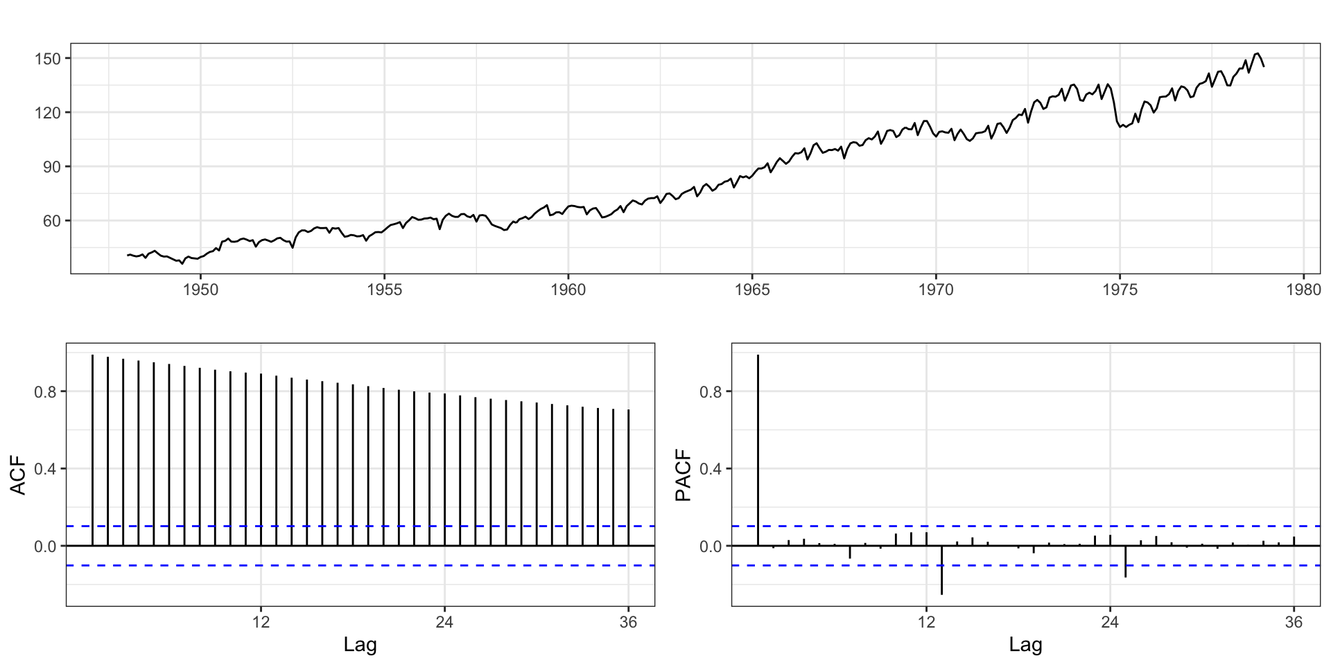
prodn from the astsa package

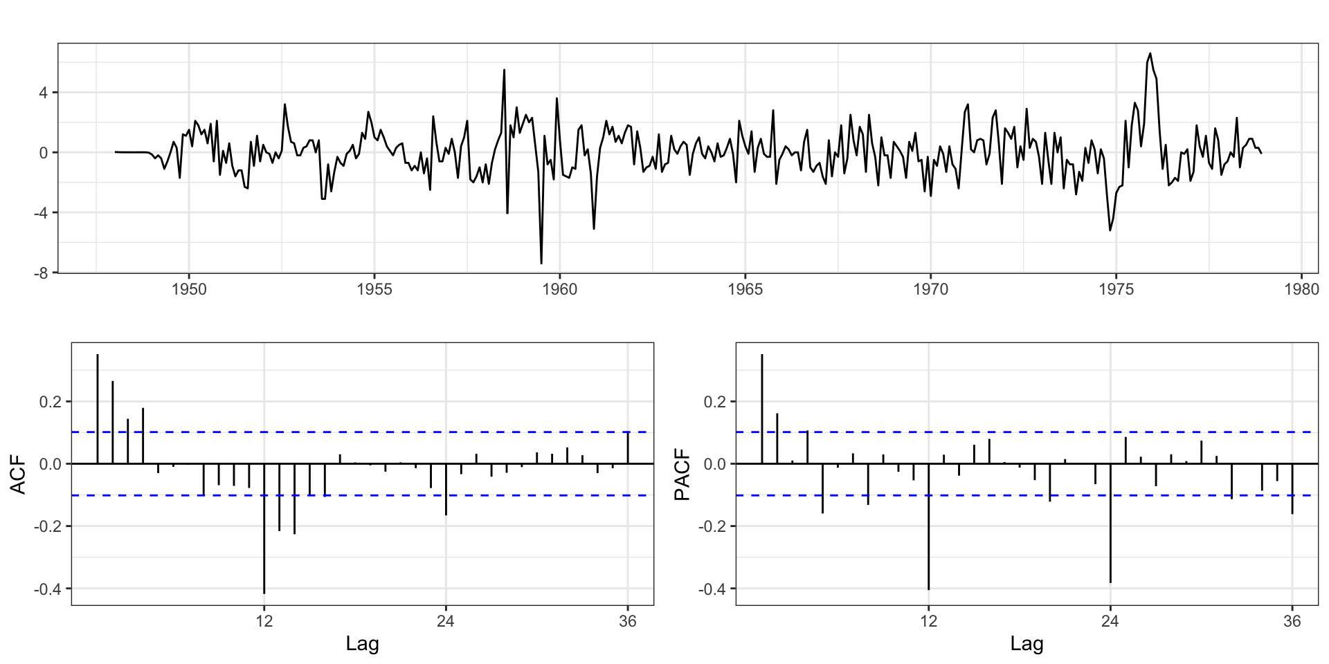
Monthly Federal Reserve Board Production Index (1948-1978)

data(prodn, package="astsa")
forecast::ggtsdisplay(prodn, points = FALSE)

Differencing

Based on the ACF it seems like standard differencing may be required

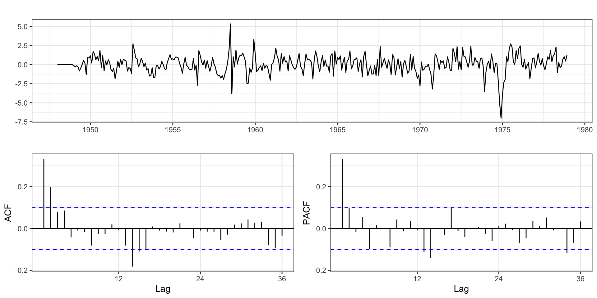
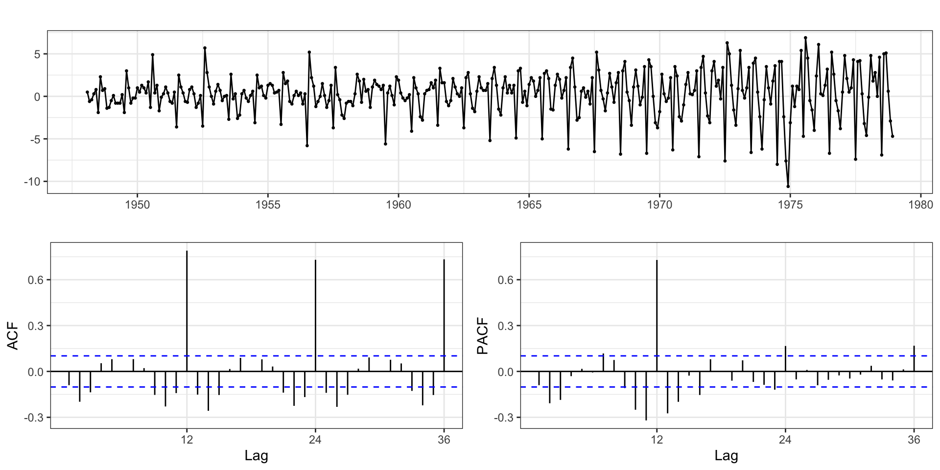
forecast::ggtsdisplay(diff(prodn))

Differencing + Seasonal Differencing

Additional seasonal differencing also seems warranted

(fr_m1 = forecast::Arima(
  prodn, order = c(0,1,0), 
  seasonal = list(order=c(0,0,0), period=12)
))
Series: prodn 
ARIMA(0,1,0) 

sigma^2 = 7.147:  log likelihood = -891.26
AIC=1784.51   AICc=1784.52   BIC=1788.43
(fr_m2 = forecast::Arima(
  prodn, order = c(0,1,0), 
  seasonal = list(order=c(0,1,0), period=12)
))
Series: prodn 
ARIMA(0,1,0)(0,1,0)[12] 

sigma^2 = 2.52:  log likelihood = -675.29
AIC=1352.58   AICc=1352.59   BIC=1356.46
yardstick::rmse_vec(
  prodn %>% unclass(), 
  fr_m1$fitted %>% unclass()
)
[1] 2.669854
yardstick::rmse_vec(
  prodn %>% unclass(), 
  fr_m2$fitted %>% unclass()
)
[1] 1.559426

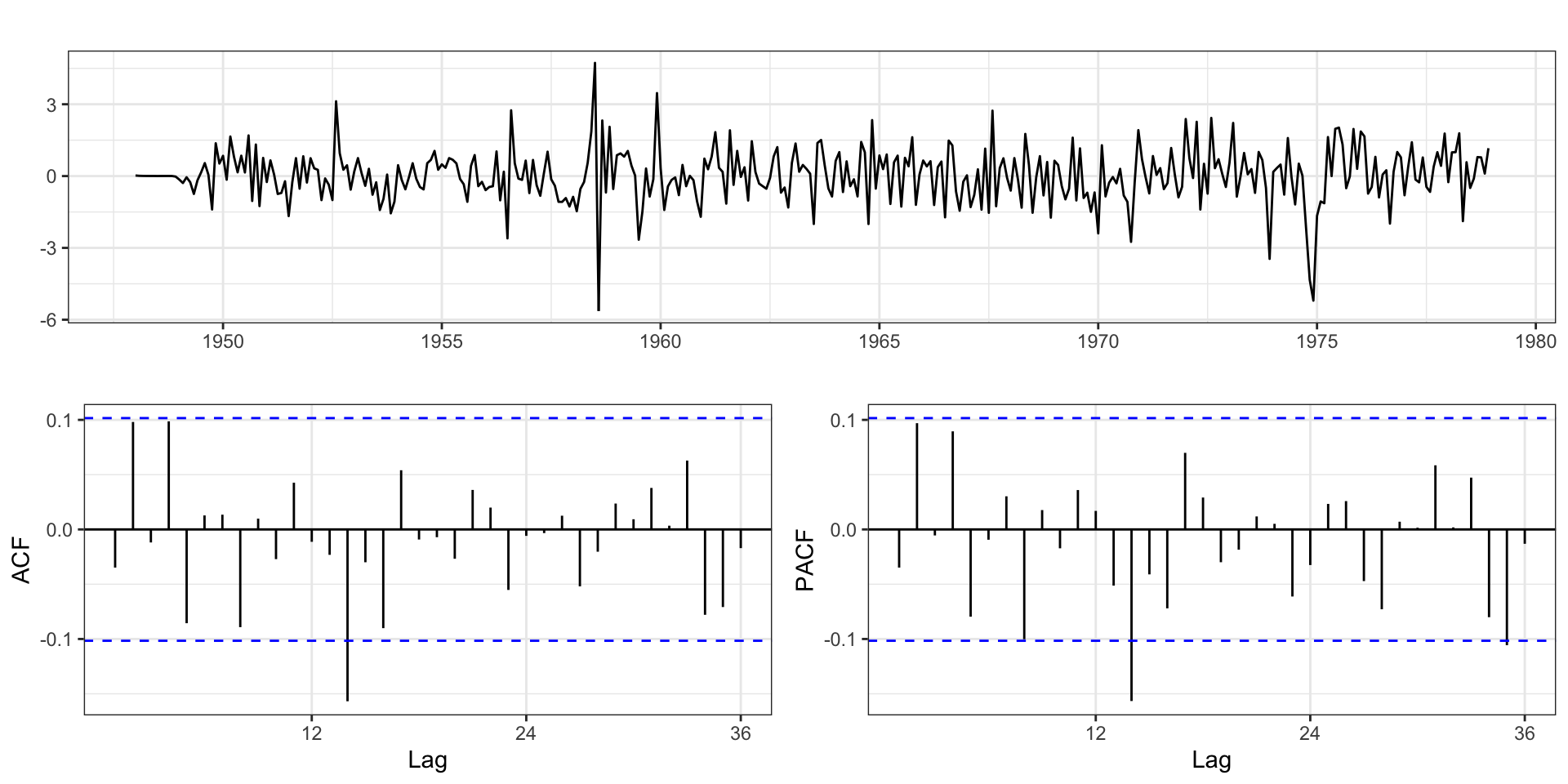
Residuals - Model 2

forecast::ggtsdisplay(fr_m2$residuals, points=FALSE, lag.max=36)

Adding Seasonal MA

(fr_m3.1 = forecast::Arima(
  prodn, order = c(0,1,0), 
  seasonal = list(order=c(0,1,1), period=12)
))
Series: prodn 
ARIMA(0,1,0)(0,1,1)[12] 

Coefficients:
         sma1
      -0.7151
s.e.   0.0317

sigma^2 = 1.616:  log likelihood = -599.29
AIC=1202.57   AICc=1202.61   BIC=1210.34
(fr_m3.2 = forecast::Arima(
  prodn, order = c(0,1,0), 
  seasonal = list(order=c(0,1,2), period=12)
))
Series: prodn 
ARIMA(0,1,0)(0,1,2)[12] 

Coefficients:
         sma1    sma2
      -0.7624  0.0520
s.e.   0.0689  0.0666

sigma^2 = 1.615:  log likelihood = -598.98
AIC=1203.96   AICc=1204.02   BIC=1215.61
yardstick::rmse_vec(
  prodn %>% unclass(), 
  fr_m3.1$fitted %>% unclass()
)
[1] 1.246885
yardstick::rmse_vec(
  prodn %>% unclass(), 
  fr_m3.2$fitted %>% unclass()
)
[1] 1.245104

Adding Seasonal MA (cont.)

(fr_m3.3 = forecast::Arima(
  prodn, order = c(0,1,0), 
  seasonal = list(order=c(0,1,3), period=12)
))
Series: prodn 
ARIMA(0,1,0)(0,1,3)[12] 

Coefficients:
         sma1     sma2    sma3
      -0.7853  -0.1205  0.2624
s.e.   0.0529   0.0644  0.0529

sigma^2 = 1.506:  log likelihood = -587.58
AIC=1183.15   AICc=1183.27   BIC=1198.69
yardstick::rmse_vec(
  prodn %>% unclass(), 
  fr_m3.3$fitted %>% unclass()
)
[1] 1.200592

Residuals - Model 3.3

Adding AR

(fr_m4.1 = forecast::Arima(
  prodn, order = c(1,1,0), 
  seasonal = list(order=c(0,1,3), period=12)
))
Series: prodn 
ARIMA(1,1,0)(0,1,3)[12] 

Coefficients:
         ar1     sma1     sma2    sma3
      0.3393  -0.7619  -0.1222  0.2756
s.e.  0.0500   0.0527   0.0646  0.0525

sigma^2 = 1.341:  log likelihood = -565.98
AIC=1141.95   AICc=1142.12   BIC=1161.37
(fr_m4.2 = forecast::Arima(
  prodn, order = c(2,1,0), 
  seasonal = list(order=c(0,1,3), period=12)
))
Series: prodn 
ARIMA(2,1,0)(0,1,3)[12] 

Coefficients:
         ar1     ar2     sma1     sma2    sma3
      0.3038  0.1077  -0.7393  -0.1445  0.2815
s.e.  0.0526  0.0538   0.0539   0.0653  0.0526

sigma^2 = 1.331:  log likelihood = -563.98
AIC=1139.97   AICc=1140.2   BIC=1163.26
yardstick::rmse_vec(
  prodn %>% unclass(), 
  fr_m4.1$fitted %>% unclass()
)
[1] 1.131115
yardstick::rmse_vec(
  prodn %>% unclass(), 
  fr_m4.2$fitted %>% unclass()
)
[1] 1.125322

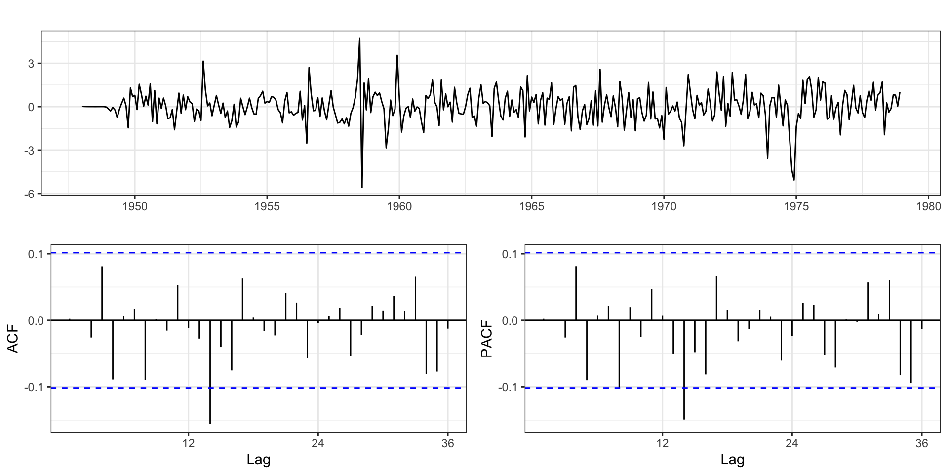
Residuals - Model 4.1

Residuals - Model 4.2
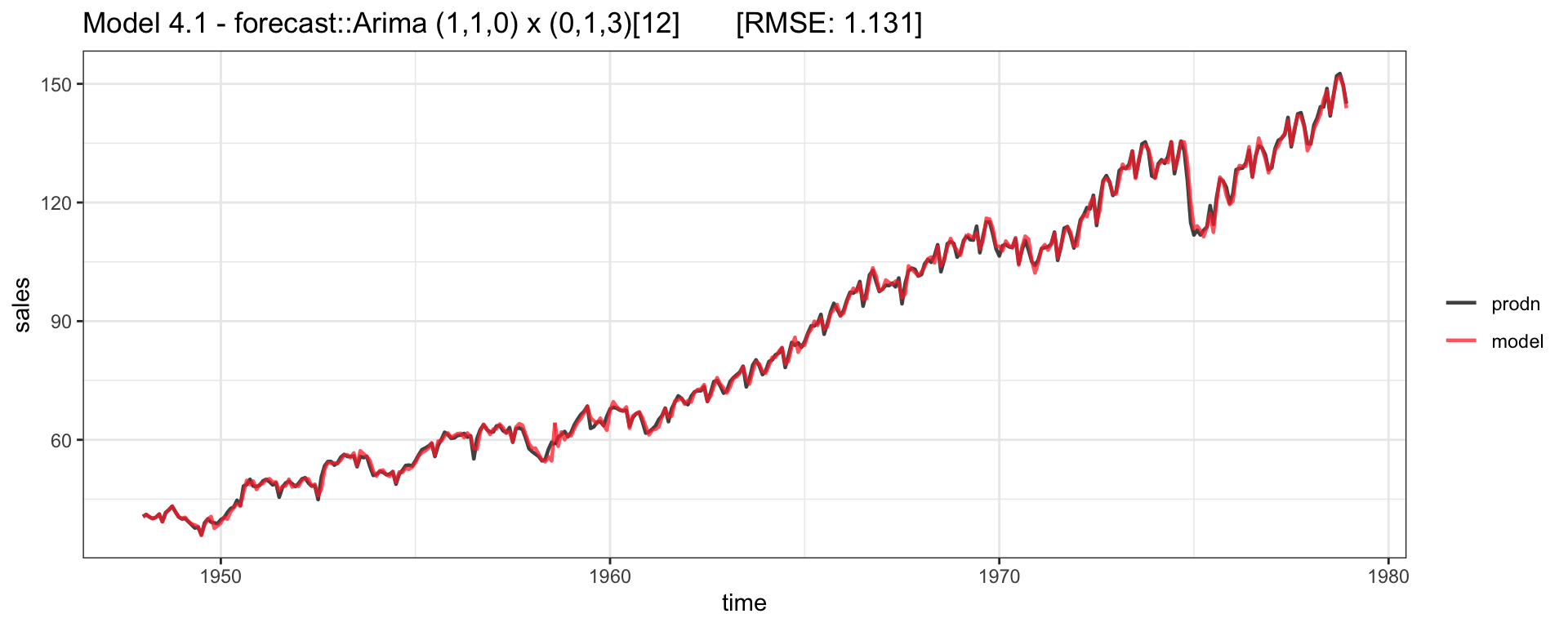
Model Fit
Model Forecast
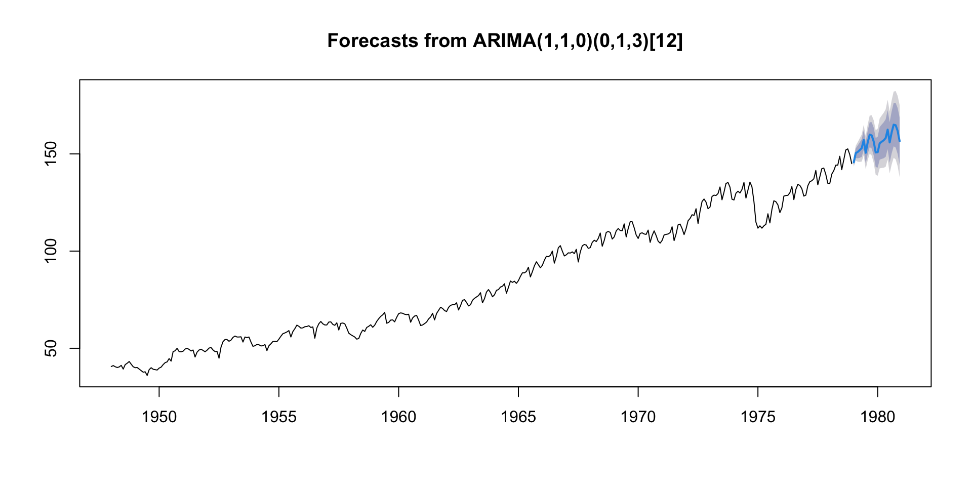
forecast::forecast(fr_m4.1) %>% plot()

Model Forecast (cont.)

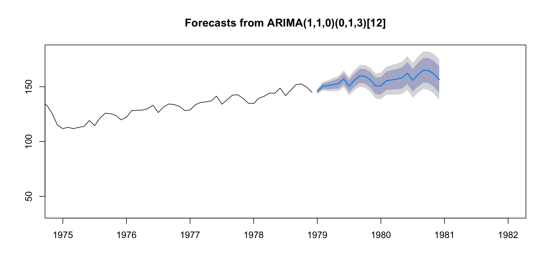
forecast::forecast(fr_m4.1) %>% plot(xlim=c(1975,1982))

Model Forecast (cont.)

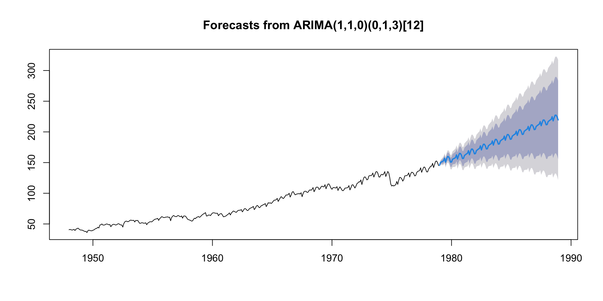
forecast::forecast(fr_m4.1, 120) %>% plot()

Model Forecast (cont.)

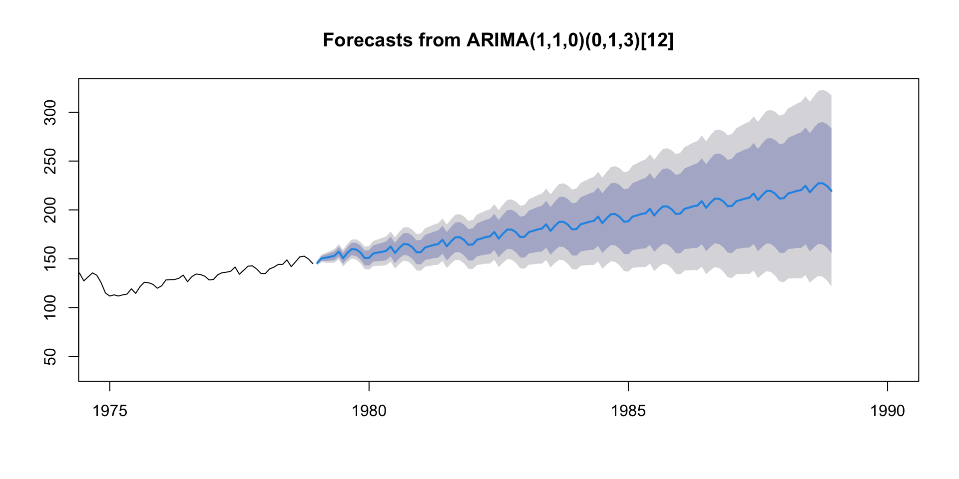
forecast::forecast(fr_m4.1, 120) %>% plot(xlim=c(1975,1990))

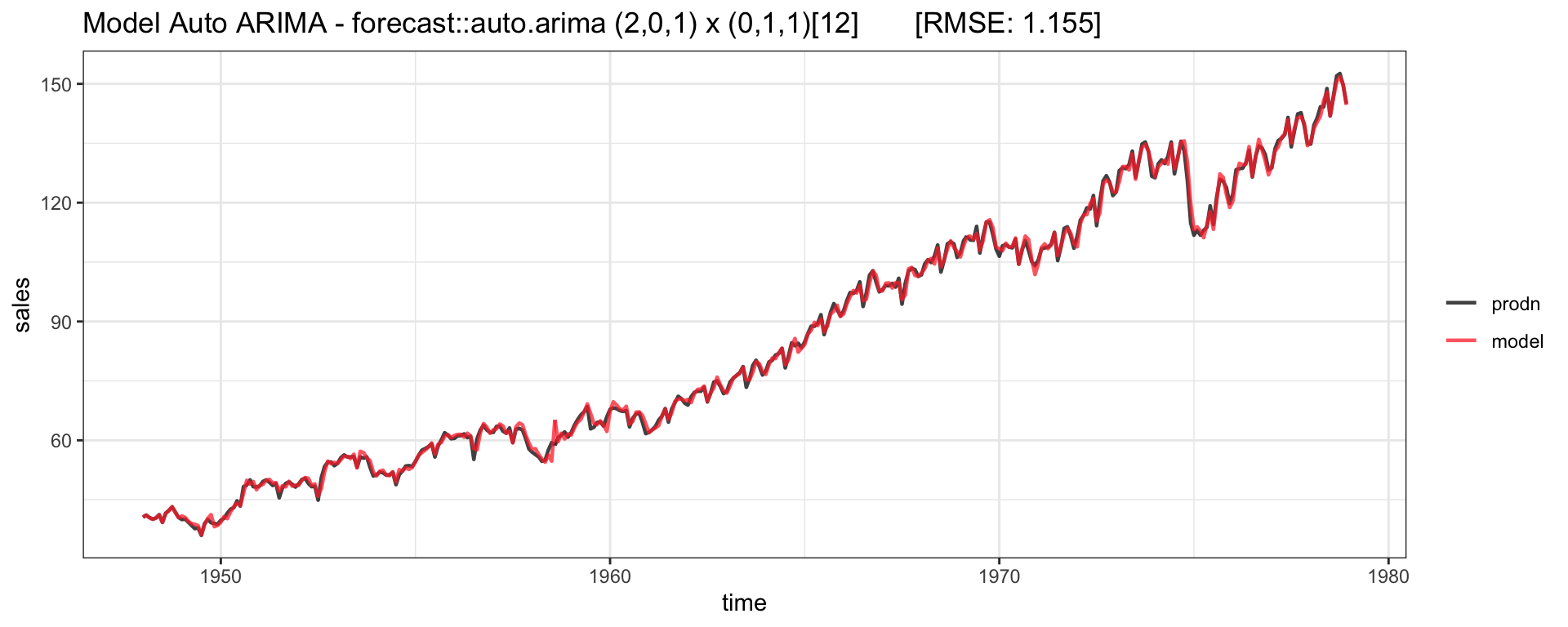
Auto ARIMA - Model Fit

Exercise - Cortecosteroid Drug Sales

Monthly cortecosteroid drug sales in Australia from 1992 to 2008.
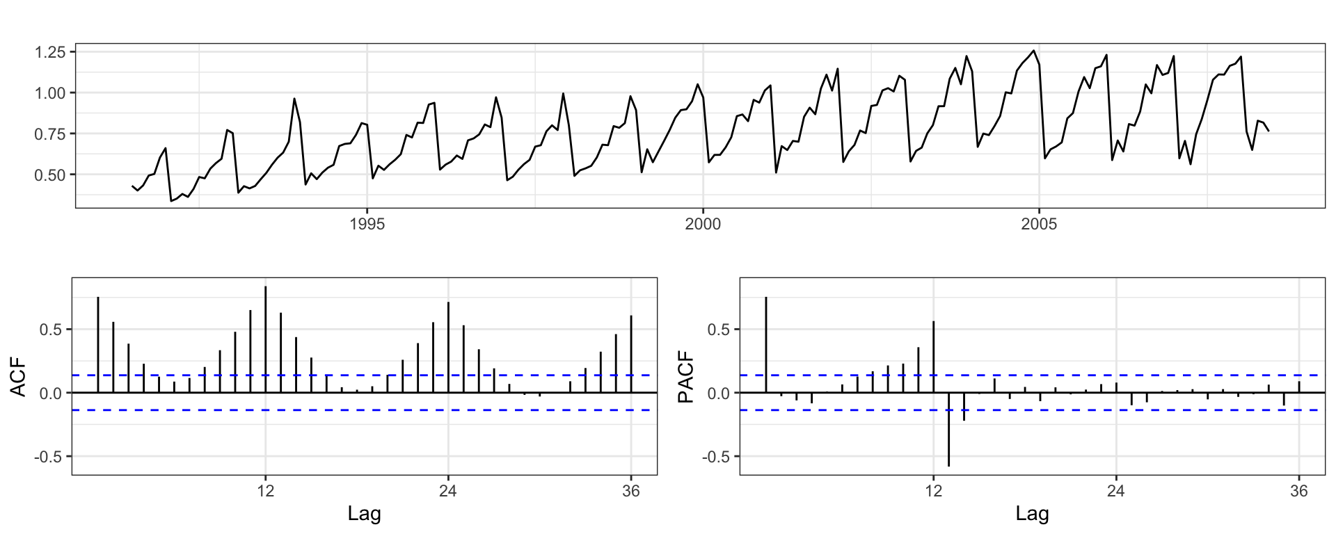
data(h02, package="fpp")
forecast::ggtsdisplay(h02, points=FALSE)