AR, MA, and ARMA Models
Lecture 09
AR models
AR(1) models
From last time we derived the following properties for AR(1) models,
\[ \begin{aligned} y_t &= \delta + \phi \, y_{t-1} + w_t \\ w_t &\overset{iid}{\sim} N(0, \sigma^2_w) \\ \end{aligned} \]
The process \(y_t\) is stationary iff \(|\phi| < 1\), and if stationary then
\[ \begin{aligned} E(y_t) &= \frac{\delta}{1-\phi} \\ Var(y_t) &= \gamma(0) = \frac{\sigma^2_w}{1-\phi^2} \\ Cov(y_t, y_{t+h}) &= \gamma(h) = \phi^h \frac{\sigma^2_w}{1-\phi^2} = \phi^h \gamma(0) \\ Corr(y_t, y_{t+h}) &= \rho(h) = \frac{\gamma(h)}{\gamma(0)} = \phi^h \end{aligned} \]
AR(p) models
We can generalize from an AR(1) to an AR(p) model by simply adding additional autoregressive terms to the model.
\[ \begin{aligned} AR(p): \quad y_t &= \delta + \phi_1 \, y_{t-1} + \phi_2 \, y_{t-2} + \cdots + \phi_p \, y_{t-p} + w_t \\ &= \delta + w_t + \sum_{i=1}^p \phi_i \, y_{t-i} \end{aligned} \]
What are the properities of \(AR(p)\), specifically
Stationarity conditions?
Expected value?
Autocovariance / autocorrelation?
Lag operator
The lag operator is convenience notation for writing out AR (and other) time series models.
We define the lag operator \(L\) as follows, \[L \, y_t = y_{t-1}\]
this can be generalized where, \[ \begin{aligned} L^2 y_t &= L\,(L\, y_{t})\\ &= L \, y_{t-1} \\ &= y_{t-2} \\ \end{aligned} \] therefore, \[L^k \, y_t = y_{t-k}\]
Lag polynomial
Lets rewrite the \(AR(p)\) model using the lag operator,
\[ \begin{aligned} y_t &= \delta + \phi_1 \, y_{t-1} + \phi_2 \, y_{t-2} + \ldots + \phi_p \, y_{t-p} + w_t \\ &= \delta + \phi_1 \, L \, y_t + \phi_2 \, L^2 \, y_t + \ldots + \phi_p \, L^p \, y_t + w_t \end{aligned} \]
If we group all of the \(y_t\) terms, we get the following
\[ \begin{aligned} \delta + w_t &= y_t - \phi_1 \, L \, y_t - \phi_2 \, L^2 \, y_t - \ldots - \phi_p \, L^p \, y_t\\ &= (1 - \phi_1 \, L - \phi_2 \, L^2 - \ldots - \phi_p \, L^p) \, y_t \end{aligned} \]
This polynomial of lags \[\phi_p(L) = (1 - \phi_1 \, L - \phi_2 \, L^2 - \cdots - \phi_p \, L^p)\] is called the characteristic polynomial of the AR process.
Stationarity of \(AR(p)\) processes
Claim: An \(AR(p)\) process is stationary if the roots of the characteristic polynomial lay outside the complex unit circle
If we define \(\lambda = 1/L\) then we can rewrite the characteristic polynomial as
\[ (\lambda^p - \phi_1 \lambda^{p-1} - \phi_2 \lambda^{p-2} - \cdots - \phi_{p-1} \lambda - \phi_p) \]
then as a corollary of our claim the \(AR(p)\) process is stationary if the roots of this new polynomial are inside the complex unit circle, i.e. \(|\lambda| < 1\).
Example AR(1)
Example AR(2)
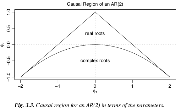
AR(2) Stationarity Conditions
Proof Sketch
We can rewrite the \(AR(p)\) model into an \(AR(1)\) form using matrix notation
\[ y_t = \delta + \phi_1 \, y_{t-1} + \phi_2 \, y_{t-2} + \cdots + \phi_p \, y_{t-p} + w_t \\ \boldsymbol\xi_t = \boldsymbol{\delta} + \boldsymbol{F} \, \boldsymbol\xi_{t-1} + \boldsymbol w_t \] where
\[ \begin{aligned} \underset{p \times 1}{\boldsymbol\xi_t} &= [y_t, y_{t-1}, y_{t-2}, \ldots, y_{t-p+1}]' \\ \underset{p \times 1}{\boldsymbol\delta} &= [\delta, 0, 0,\ldots, 0]'\\ \underset{p \times 1}{\boldsymbol{w}_{t}} &= [w_t, 0, 0,\ldots, 0]' \\ \end{aligned} \]
\[ \begin{aligned} \underset{p \times p}{\boldsymbol{F}} &= \begin{bmatrix} \phi_1 & \phi_2 & \phi_3 & \cdots & \phi_{p-1} & \phi_p \\ 1 & 0 & 0 & \cdots & 0 & 0 \\ 0 & 1 & 0 & \cdots & 0 & 0 \\ \vdots & \vdots & \vdots & \cdots & \vdots & \vdots \\ 0 & 0 & 0 & \cdots & 1 & 0 \\ \end{bmatrix} \end{aligned} \]
Putting it together
Proof sketch (cont.)
So just like the original \(AR(1)\) we can expand out the autoregressive equation
\[ \begin{aligned} \boldsymbol\xi_t &= \boldsymbol{\delta} + \boldsymbol w_t + \boldsymbol{F} \, \boldsymbol\xi_{t-1} \\ &= \boldsymbol{\delta} + \boldsymbol w_t + \boldsymbol{F} \, (\boldsymbol\delta+\boldsymbol w_{t-1}) + \boldsymbol{F}^2 \, (\boldsymbol \delta+\boldsymbol w_{t-2}) + \cdots \\ &\qquad\qquad~\,\,\, + \boldsymbol{F}^{t-1} \, (\boldsymbol \delta+\boldsymbol w_{1}) + \boldsymbol{F}^t \, (\boldsymbol \delta+\boldsymbol w_0) \\ &= \left(\sum_{i=0}^t F^i\right)\boldsymbol{\delta} + \sum_{i=0}^t F^i \, w_{t-i} \end{aligned} \]
and therefore we need \(\underset{t\to\infty}{\lim} F^t \to 0\) so that \(\underset{t\to\infty}{\lim} \sum_{i=0}^t F^i < \infty\).
Proof sketch (cont.)
We can find the eigen decomposition such that \(\boldsymbol F = \boldsymbol Q \boldsymbol \Lambda \boldsymbol Q^{-1}\) where the columns of \(\boldsymbol Q\) are the eigenvectors of \(\boldsymbol F\) and \(\boldsymbol \Lambda\) is a diagonal matrix of the corresponding eigenvalues.
A useful property of the eigen decomposition is that
\[ \boldsymbol{F}^i = \boldsymbol Q \boldsymbol \Lambda^i \boldsymbol Q^{-1} \]
Using this property we can rewrite our equation from the previous slide as
\[ \begin{aligned} \boldsymbol\xi_t &= (\sum_{i=0}^t F^i)\boldsymbol{\delta} + \sum_{i=0}^t F^i \, w_{t-i} \\ &= \left(\sum_{i=0}^t \boldsymbol Q \boldsymbol \Lambda^i \boldsymbol Q^{-1}\right)\boldsymbol{\delta} + \sum_{i=0}^t \boldsymbol Q \boldsymbol \Lambda^i \boldsymbol Q^{-1} \, w_{t-i} \end{aligned} \]
Proof sketch (cont.)
\[ \boldsymbol \Lambda^i = \begin{bmatrix} \lambda_1^i & 0 & \cdots & 0 \\ 0 & \lambda_2^i & \cdots & 0 \\ \vdots & \vdots & \ddots & \vdots \\ 0 & 0 & \cdots & \lambda_p^i \\ \end{bmatrix} \]
Therefore, \(\underset{t\to\infty}{\lim} F^t \to 0\) when \(\underset{t\to\infty}{\lim} \Lambda^t \to 0\) which requires that \[|\lambda_i| < 1 \;\; \text{ for all} \; i\]
Proof sketch (cont.)
Eigenvalues are defined such that for \(\boldsymbol \lambda\),
\[ \det (\boldsymbol{F}-\boldsymbol\lambda\,\boldsymbol{I}) = 0\]
based on our definition of \(\boldsymbol F\) our eigenvalues will therefore be the roots of
\[\lambda^p -\phi_1\,\lambda^{p-1}-\phi_2\,\lambda^{p-2} - \cdots - \phi_{p_1} \, \lambda^1 - \phi_p = 0\]
which if we multiply by \(1/\lambda^p\) where \(L = 1/\lambda\) gives
\[1 -\phi_1\,L-\phi_2\,L^2 - \cdots - \phi_{p_1} \, L^{p-1} - \phi_p \, L^p = 0\]
Properties of \(AR(2)\)
For a stationary \(AR(2)\) process,
Properties of \(AR(2)\) (cont.)
Properties of \(AR(p)\)
For a stationary \(AR(p)\) process,
\[ E(Y_t) = \frac{\delta}{1-\phi_1 -\phi_2-\ldots-\phi_p} \]
\[ Var(y_t) = \gamma(0) = \phi_1\gamma(1) + \phi_2\gamma(2) + \ldots + \phi_p\gamma(p) + \sigma_w^2 \\ \]
\[ Cov(y_t, y_{t+h}) = \gamma(h) = \phi_1\gamma(h-1) + \phi_2\gamma(h-2) + \ldots + \phi_p\gamma(h-p) \]
\[ Corr(y_t, y_{t+h}) = \rho(h) = \phi_1\,\rho(h-1) + \phi_2\,\rho(h-2) + \ldots + \phi_p\,\rho(h-p) \]
Moving Average (MA) Processes
MA(1)
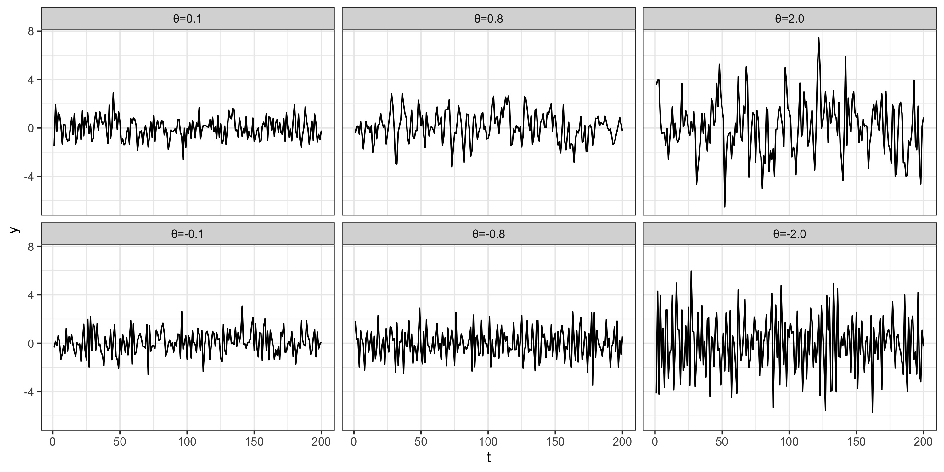
A moving average process is similar to an AR process, except that the autoregression is on the error term. \[ MA(1): \qquad y_t = \delta + w_t + \theta \, w_{t-1} \]
Properties:
MA(1) - properties (cont.)
Time series
ACF

MA(q)
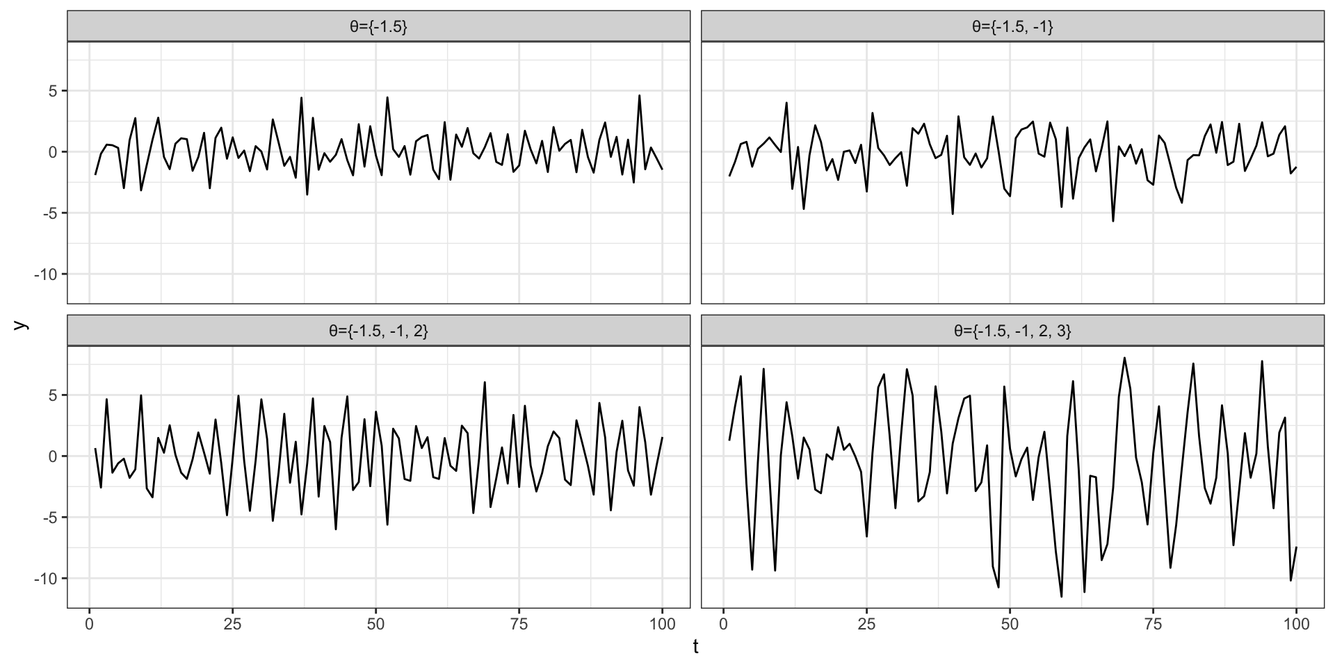
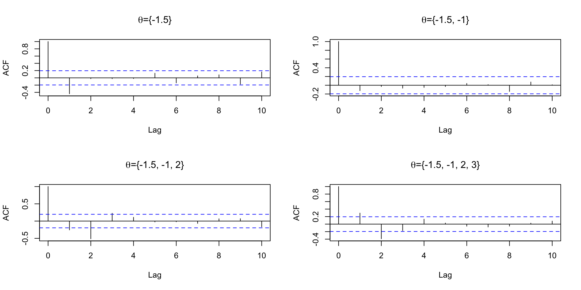
\[ MA(q): \qquad y_t = \delta + w_t + \theta_1 \, w_{t-1} + \theta_2 \, w_{t-2} + \cdots + \theta_q \, w_{t-q} \]
Properties:
\[E(y_t) = \delta\]
\[ \begin{aligned} Var(y_t) = \gamma(0) &= (1 + \theta_1^2+\theta_2^2 + \cdots + \theta_q^2) \, \sigma_w^2 \\ \\ Cov(y_t, y_{t+h}) = \gamma(h) &= \begin{cases} \sigma^2 \sum_{j=0}^{q-|h|} \theta_j \theta_{j+|h|} & \text{if $|h| \leq q$} \\ 0 & \text{if $|h| > q$} \end{cases} \end{aligned} \]
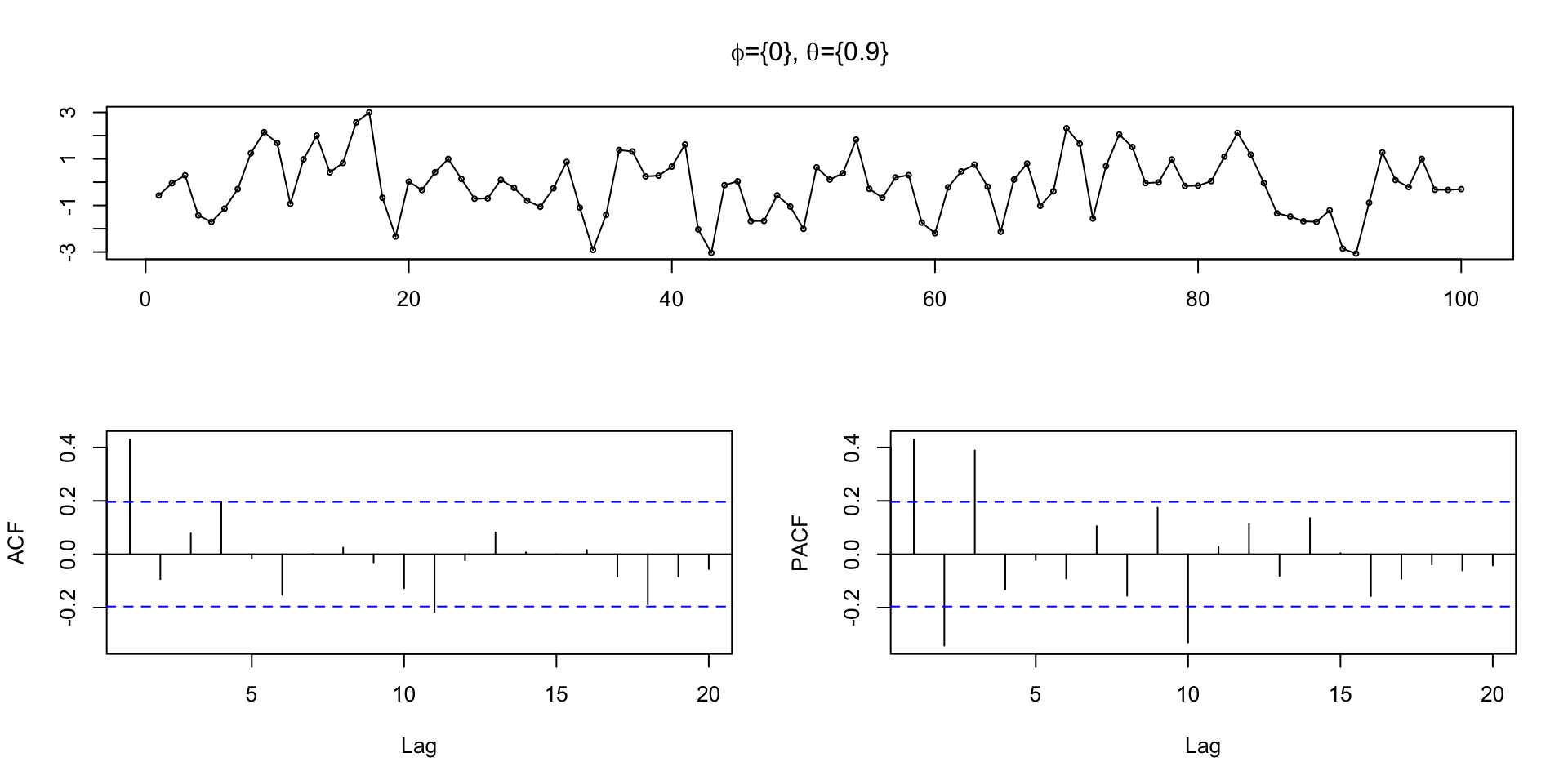
Example series
ACF
PACF

ARMA Model
ARMA Model
An ARMA model is a composite of AR and MA processes,
\(ARMA(p,q)\): \[ y_t = \delta + \phi_1 \, y_{t-1} + \cdots \phi_p \, y_{t-p} + w_{t} + \theta_1 w_{t-1} + \cdots + \theta_q w_{t_q} \] \[ \phi_p(L) y_t = \delta + \theta_q(L)w_t \]
Since all MA processes are stationary, we only need to examine the AR component to determine stationarity, i.e. check roots of \(\phi_p(L)\) lie outside the complex unit circle.
Time series
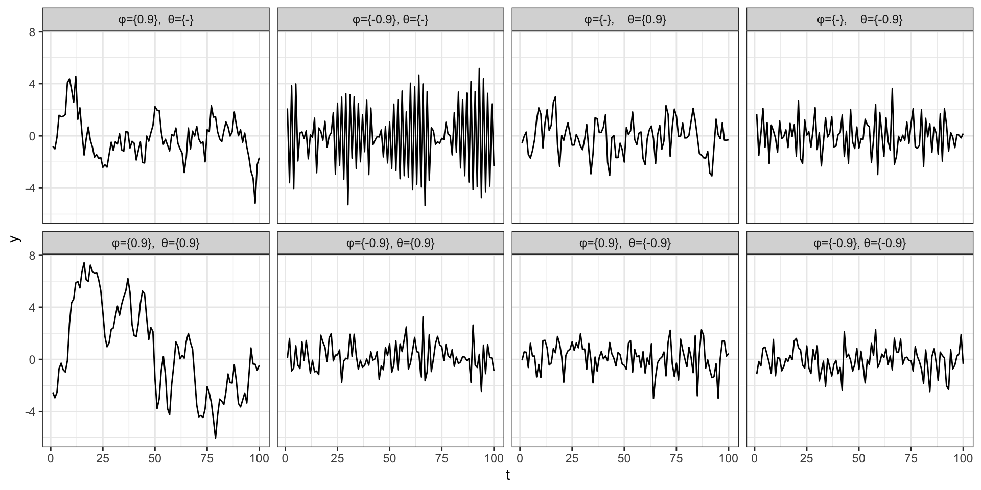
\(\phi=0.9\), \(\theta=0\)

\(\phi=0\), \(\theta=0.9\)
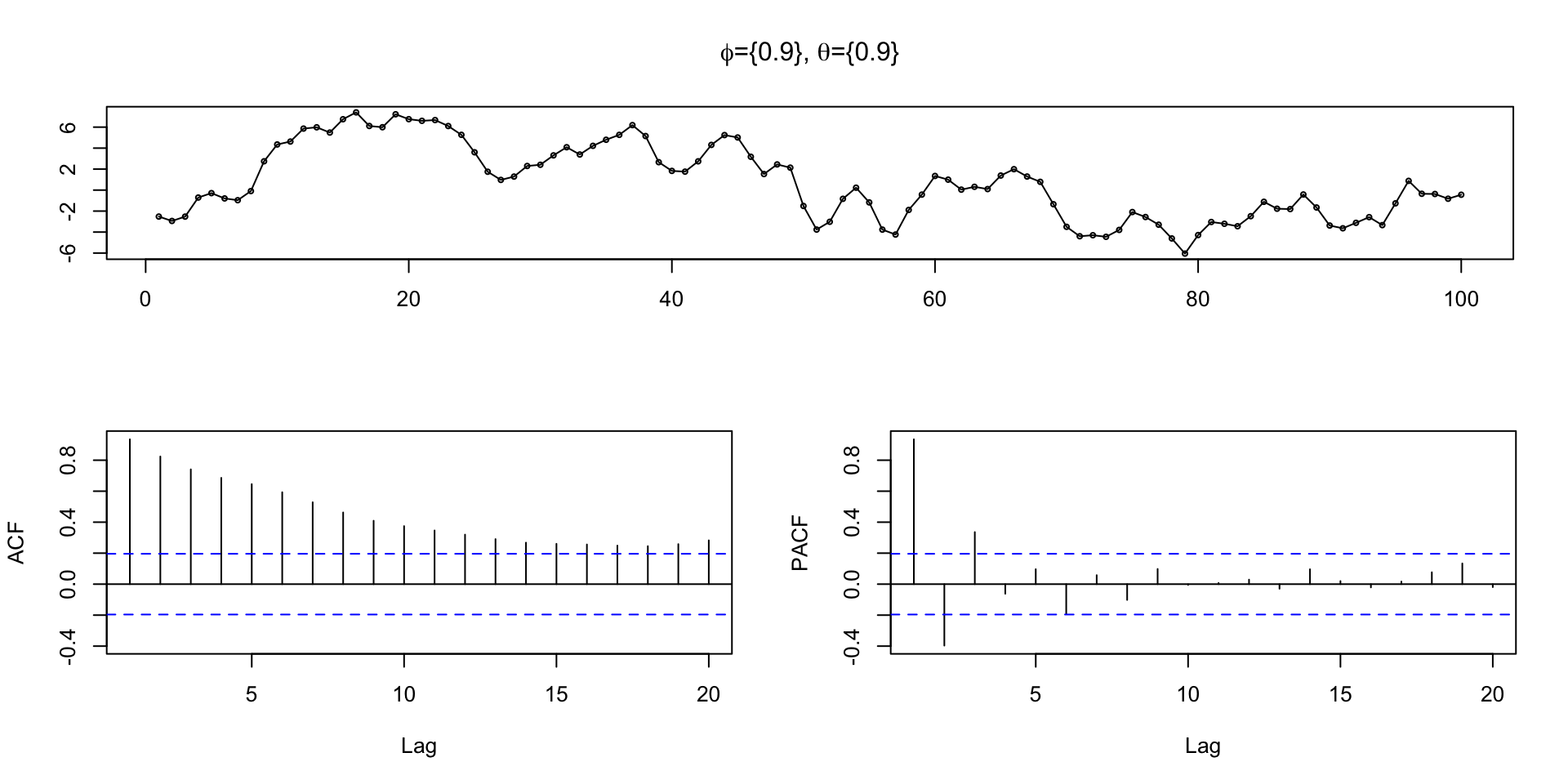
\(\phi=0.9\), \(\theta=0.9\)
Sta 344 - Fall 2022