CCFs, Differencing, & AR(1) models

Lecture 08

Dr. Colin Rundel

Lagged Predictors and CCFs

Southern Oscillation Index & Recruitment

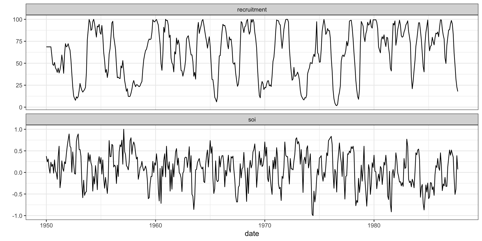
The Southern Oscillation Index (SOI) is an indicator of the development and intensity of El Niño (negative SOI) or La Niña (positive SOI) events in the Pacific Ocean. These data also included the estimate of “recruitment”, which indicate fish population sizes in the southern hemisphere.

# A tibble: 453 × 3
    date    soi recruitment
   <dbl>  <dbl>       <dbl>
 1 1950   0.377        68.6
 2 1950.  0.246        68.6
 3 1950.  0.311        68.6
 4 1950.  0.104        68.6
 5 1950. -0.016        68.6
 6 1950.  0.235        68.6
 7 1950.  0.137        59.2
 8 1951.  0.191        48.7
 9 1951. -0.016        47.5
10 1951.  0.29         50.9
# … with 443 more rows

Time series

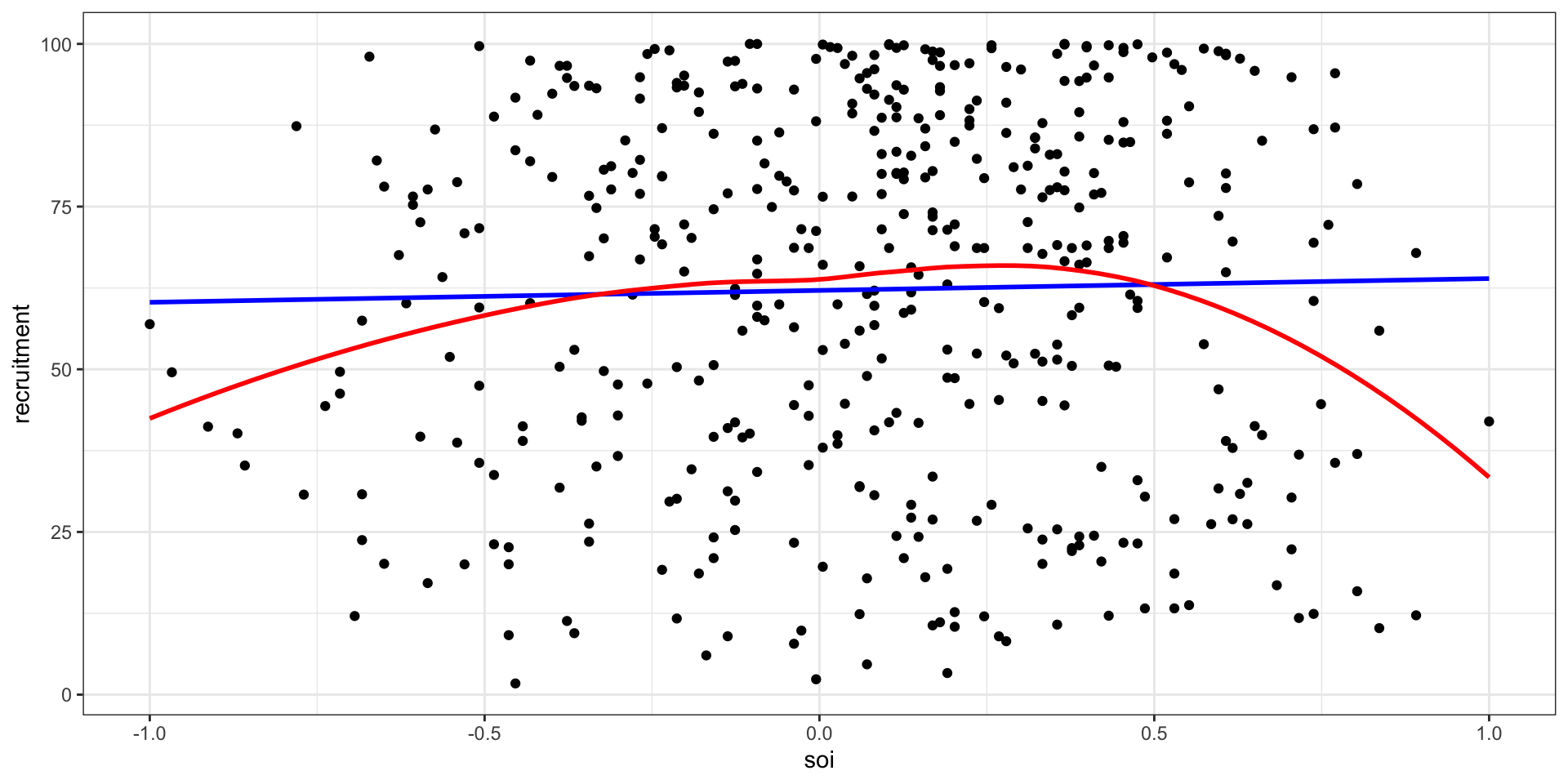
Relationship?

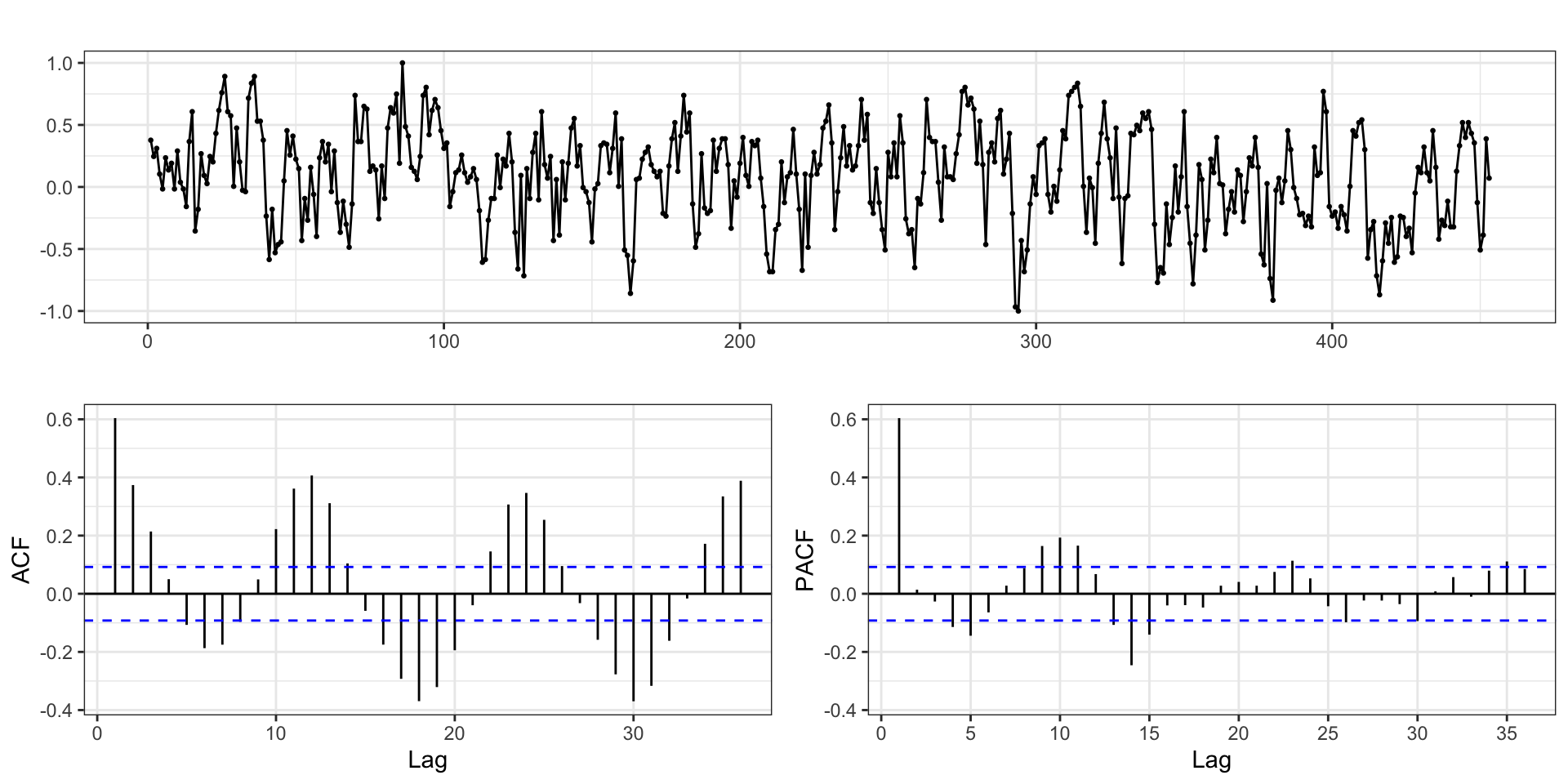
`soi` - ACF & PACF

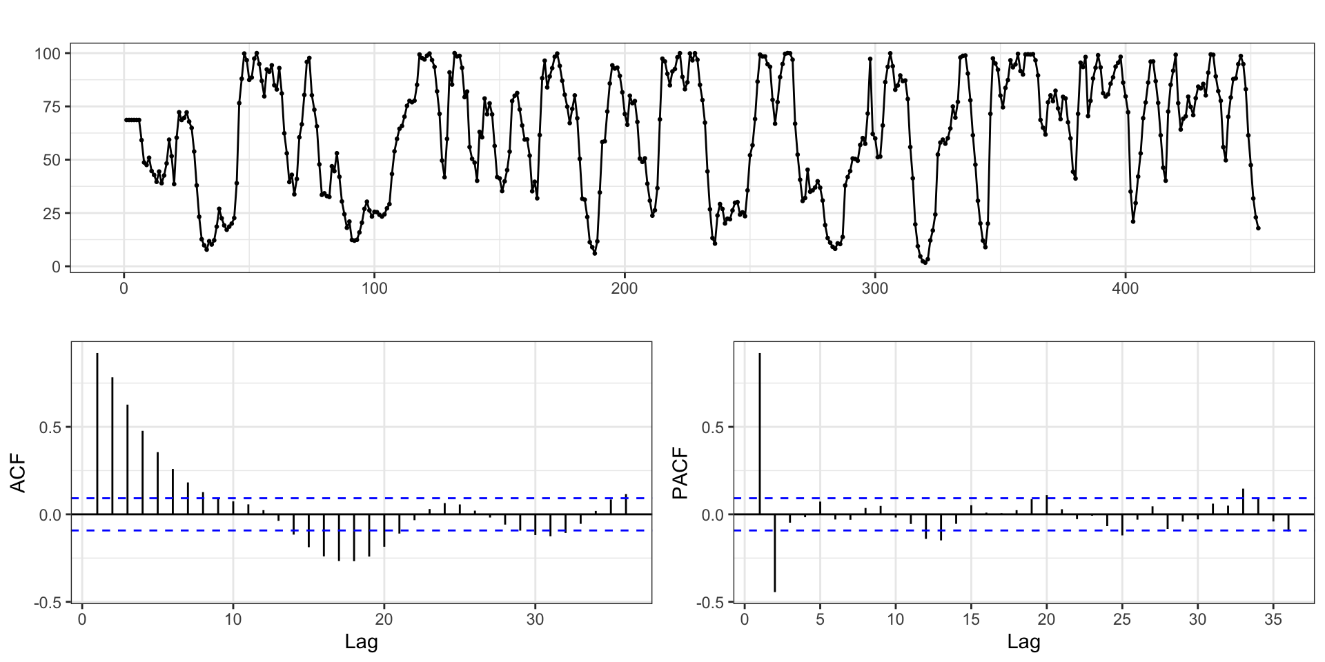
forecast::ggtsdisplay(fish$soi, lag.max = 36)

`recruitment` - ACF & PACF

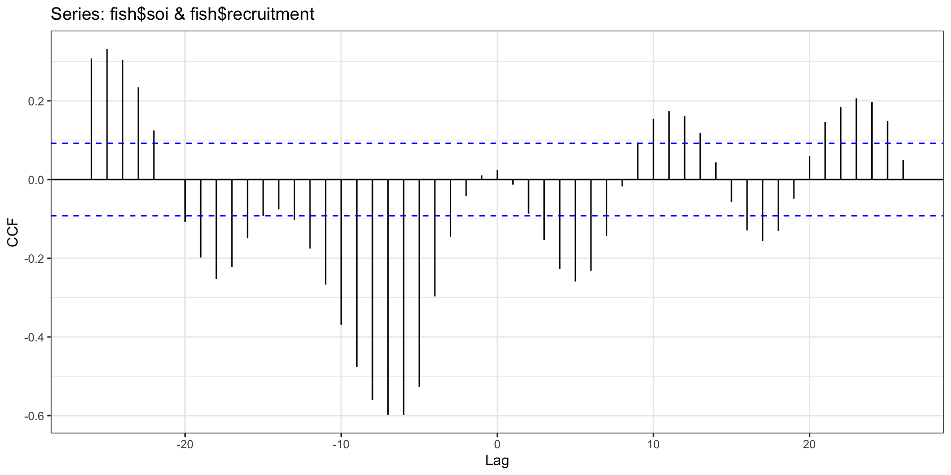
forecast::ggtsdisplay(fish$recruitment, lag.max = 36)

Cross correlation function

forecast::ggCcf(fish$soi, fish$recruitment)

Cross correlation function - Scatter plots

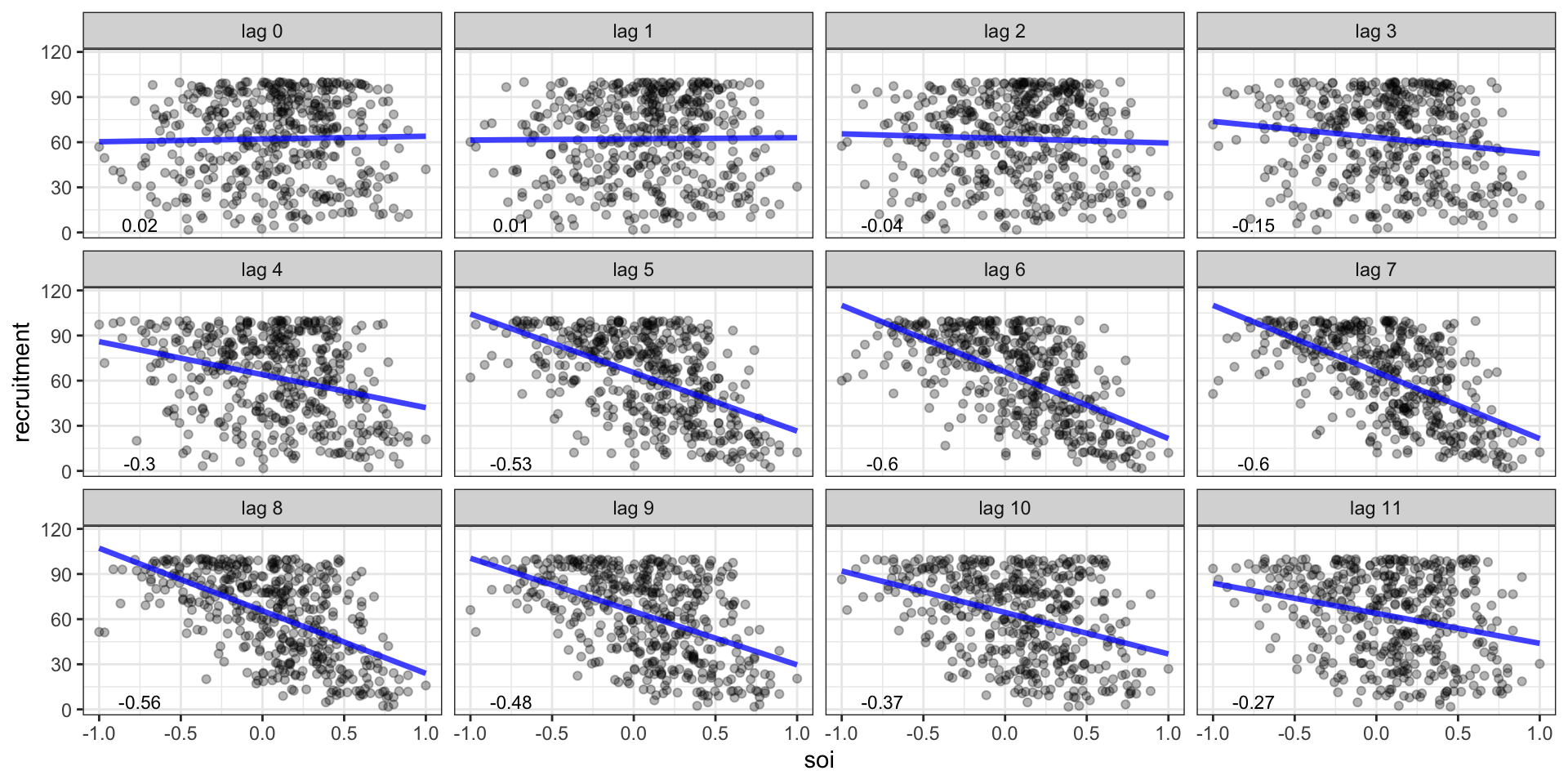
The CCF gave us negative lags, why are we not considering them here?

Model

model1 = lm(recruitment~lag(soi,6), data=fish)
model2 = lm(recruitment~lag(soi,6)+lag(soi,7), data=fish)
model3 = lm(recruitment~lag(soi,5)+lag(soi,6)+lag(soi,7)+lag(soi,8), data=fish)

summary(model3)


Call:
lm(formula = recruitment ~ lag(soi, 5) + lag(soi, 6) + lag(soi, 
    7) + lag(soi, 8), data = fish)

Residuals:
    Min      1Q  Median      3Q     Max 
-72.409 -13.527   0.191  12.851  46.040 

Coefficients:
            Estimate Std. Error t value Pr(>|t|)    
(Intercept)  67.9438     0.9306  73.007  < 2e-16 ***
lag(soi, 5) -19.1502     2.9508  -6.490 2.32e-10 ***
lag(soi, 6) -15.6894     3.4334  -4.570 6.36e-06 ***
lag(soi, 7) -13.4041     3.4332  -3.904 0.000109 ***
lag(soi, 8) -23.1480     2.9530  -7.839 3.46e-14 ***
---
Signif. codes:  0 '***' 0.001 '**' 0.01 '*' 0.05 '.' 0.1 ' ' 1

Residual standard error: 18.93 on 440 degrees of freedom
  (8 observations deleted due to missingness)
Multiple R-squared:  0.5539,    Adjusted R-squared:  0.5498 
F-statistic: 136.6 on 4 and 440 DF,  p-value: < 2.2e-16

Prediction

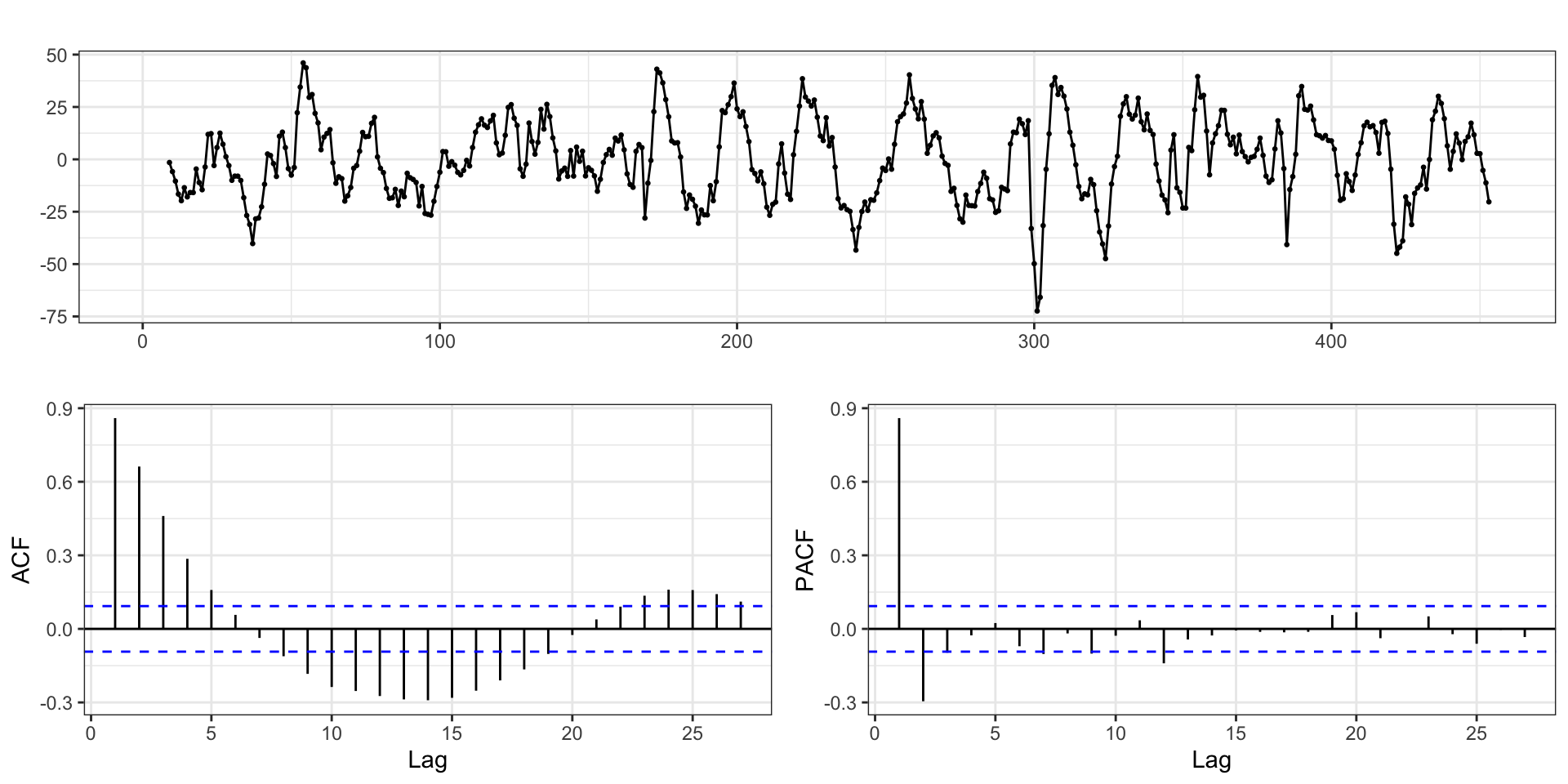
Residual ACF - Model 3

Autoregessive model 4

model4 = lm(
  recruitment~lag(recruitment,1) + lag(recruitment,2) + 
              lag(soi,5)+lag(soi,6)+lag(soi,7)+lag(soi,8), 
  data=fish
)
summary(model4)


Call:
lm(formula = recruitment ~ lag(recruitment, 1) + lag(recruitment, 
    2) + lag(soi, 5) + lag(soi, 6) + lag(soi, 7) + lag(soi, 8), 
    data = fish)

Residuals:
    Min      1Q  Median      3Q     Max 
-51.996  -2.892   0.103   3.117  28.579 

Coefficients:
                     Estimate Std. Error t value Pr(>|t|)    
(Intercept)          10.25007    1.17081   8.755  < 2e-16 ***
lag(recruitment, 1)   1.25301    0.04312  29.061  < 2e-16 ***
lag(recruitment, 2)  -0.39961    0.03998  -9.995  < 2e-16 ***
lag(soi, 5)         -20.76309    1.09906 -18.892  < 2e-16 ***
lag(soi, 6)           9.71918    1.56265   6.220 1.16e-09 ***
lag(soi, 7)          -1.01131    1.31912  -0.767   0.4437    
lag(soi, 8)          -2.29814    1.20730  -1.904   0.0576 .  
---
Signif. codes:  0 '***' 0.001 '**' 0.01 '*' 0.05 '.' 0.1 ' ' 1

Residual standard error: 7.042 on 438 degrees of freedom
  (8 observations deleted due to missingness)
Multiple R-squared:  0.9385,    Adjusted R-squared:  0.9377 
F-statistic:  1115 on 6 and 438 DF,  p-value: < 2.2e-16

Autoregessive model 5

model5 = lm(
  recruitment~lag(recruitment,1) + lag(recruitment,2) + 
              lag(soi,5) + lag(soi,6),
  data=fish
)
summary(model5)


Call:
lm(formula = recruitment ~ lag(recruitment, 1) + lag(recruitment, 
    2) + lag(soi, 5) + lag(soi, 6), data = fish)

Residuals:
    Min      1Q  Median      3Q     Max 
-53.786  -2.999  -0.035   3.031  27.669 

Coefficients:
                     Estimate Std. Error t value Pr(>|t|)    
(Intercept)           8.78498    1.00171   8.770  < 2e-16 ***
lag(recruitment, 1)   1.24575    0.04314  28.879  < 2e-16 ***
lag(recruitment, 2)  -0.37193    0.03846  -9.670  < 2e-16 ***
lag(soi, 5)         -20.83776    1.10208 -18.908  < 2e-16 ***
lag(soi, 6)           8.55600    1.43146   5.977 4.68e-09 ***
---
Signif. codes:  0 '***' 0.001 '**' 0.01 '*' 0.05 '.' 0.1 ' ' 1

Residual standard error: 7.069 on 442 degrees of freedom
  (6 observations deleted due to missingness)
Multiple R-squared:  0.9375,    Adjusted R-squared:  0.937 
F-statistic:  1658 on 4 and 442 DF,  p-value: < 2.2e-16

Prediction

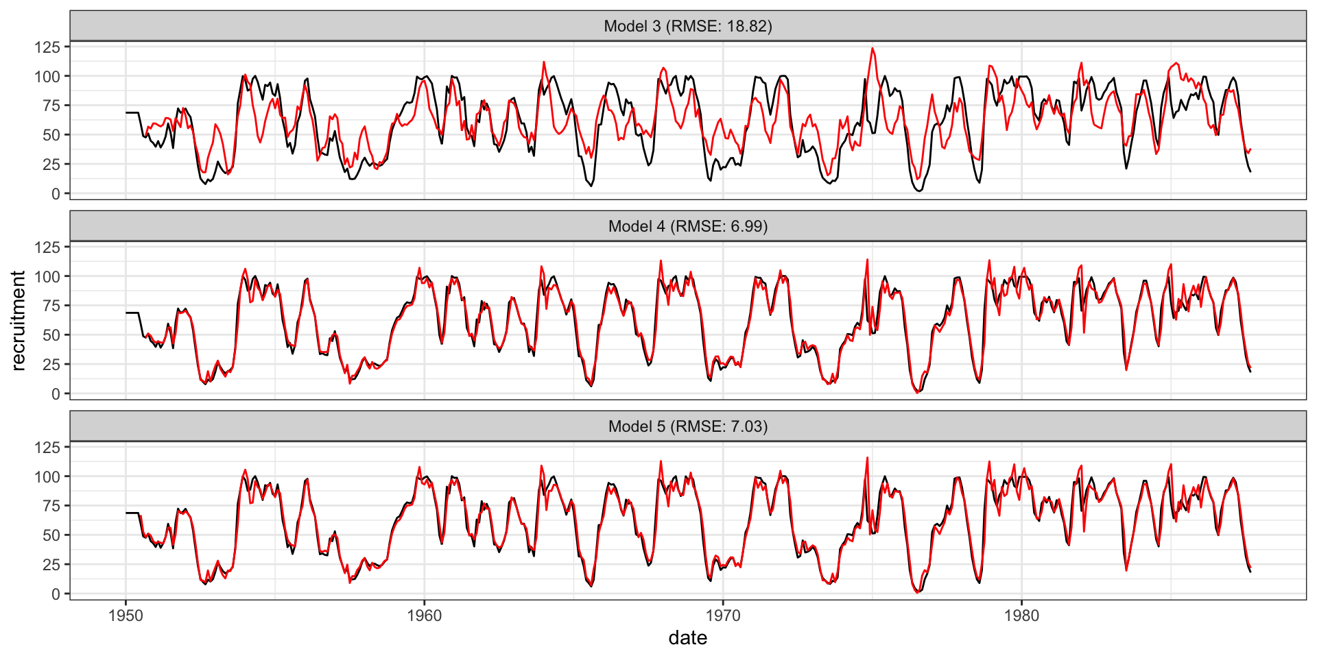
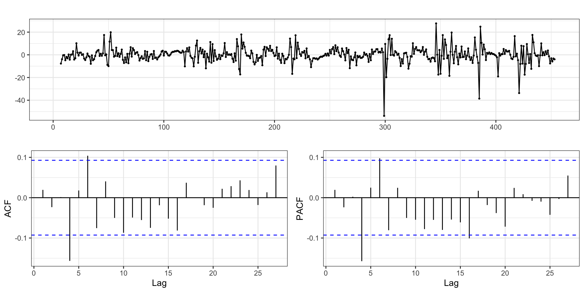
Residual ACF - Model 5

broom::augment(model5, newdata=fish) %>%
  pull(.resid) %>%
  forecast::ggtsdisplay()

Non-stationarity

Non-stationary models

All happy families are alike; each unhappy family is unhappy in its own way.

Tolstoy, Anna Karenina

This applies to time series models as well, just replace happy family with stationary model.

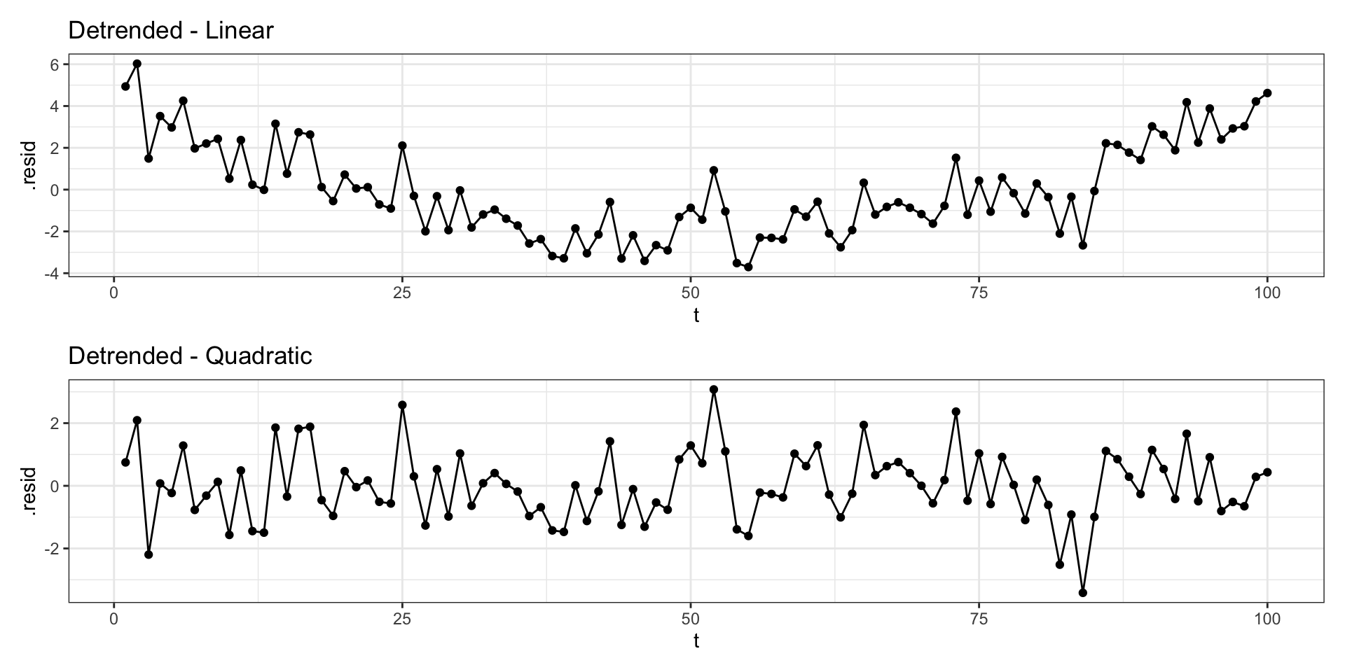
A simple example of a non-stationary time series is a trend stationary model

\[ y_t = \mu(t) + w_t \]

where \(\mu(t)\) denotes a time dependent trend and \(w_t\) is a white noise (stationary) process.

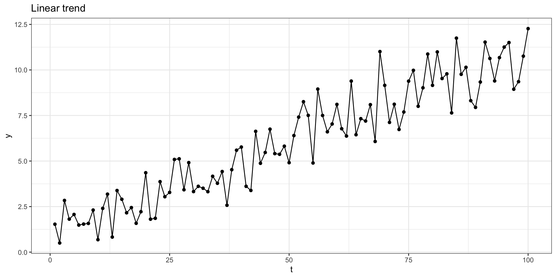
Linear trend model

Lets imagine a simple model where \(y_t = \delta + \beta t + x_t\) where \(\delta\) and \(\beta\) are constants and \(x_t\) is a stationary process.

Differencing

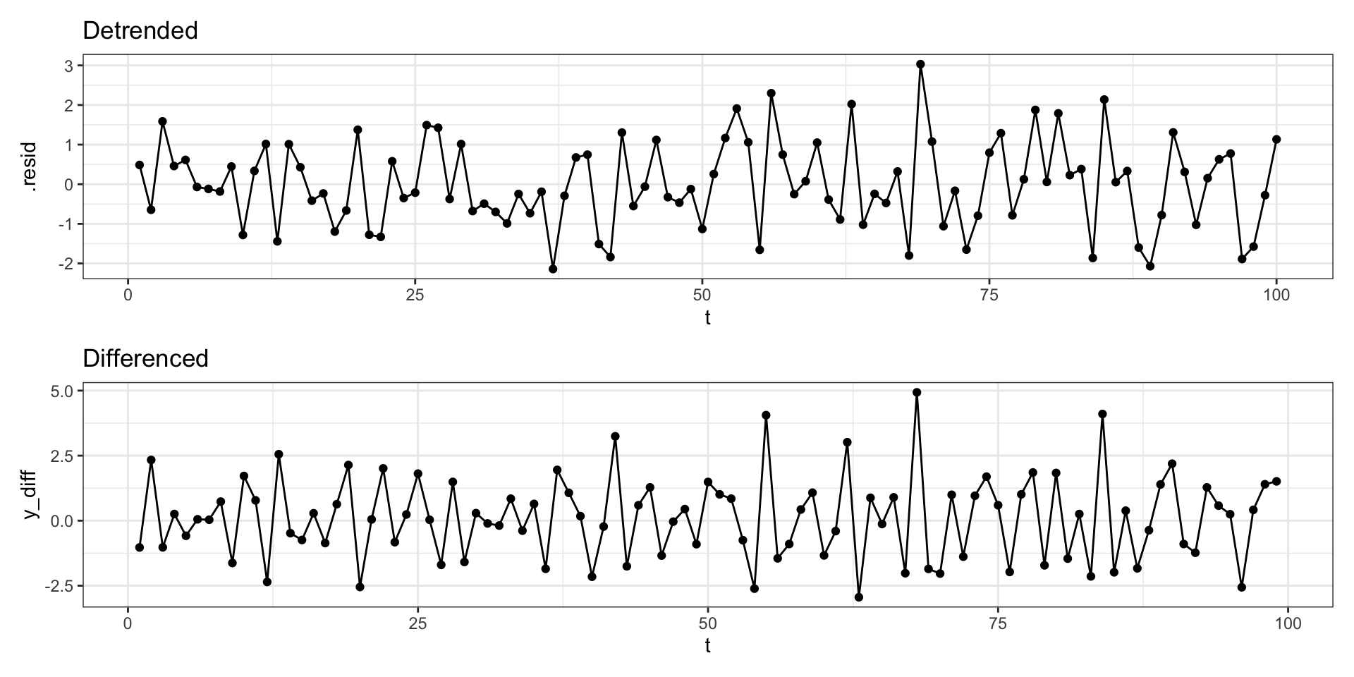
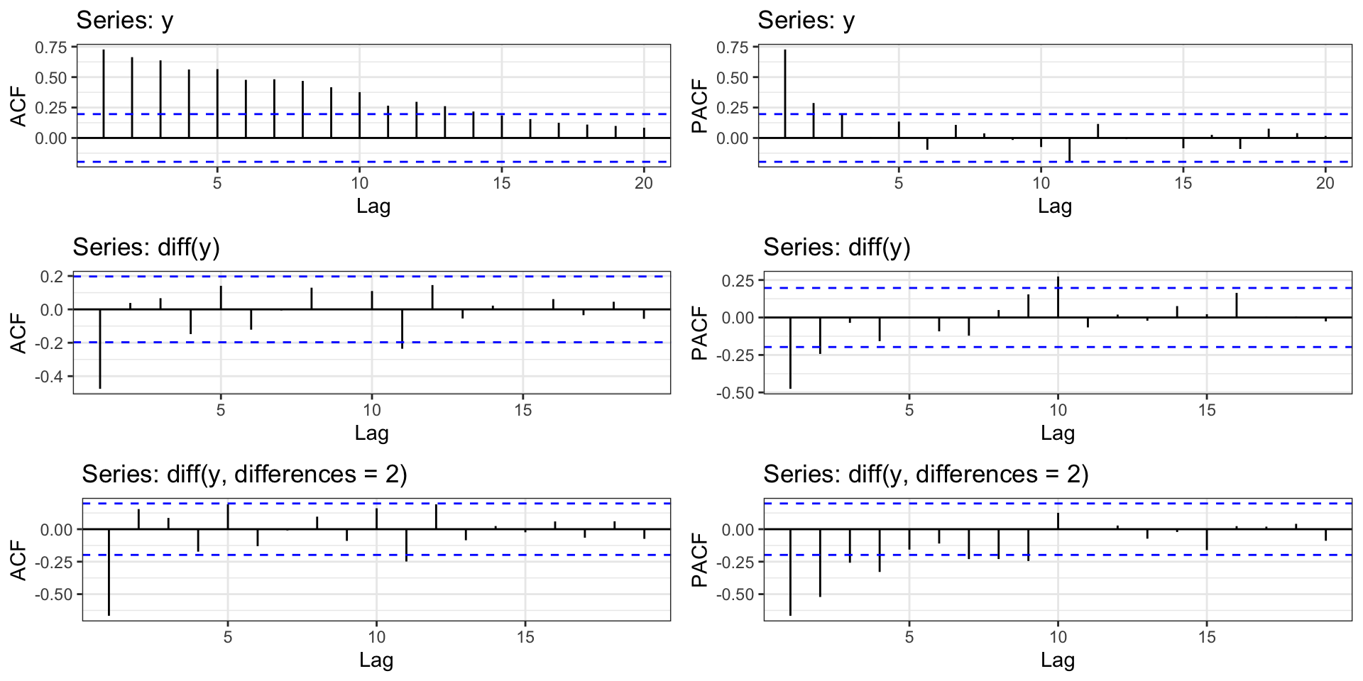
An simple approach to remove trend is to difference your response variable, specifically examine \(d_t = y_t - y_{t-1}\) instead of \(y_t\).

Detrending vs Differencing

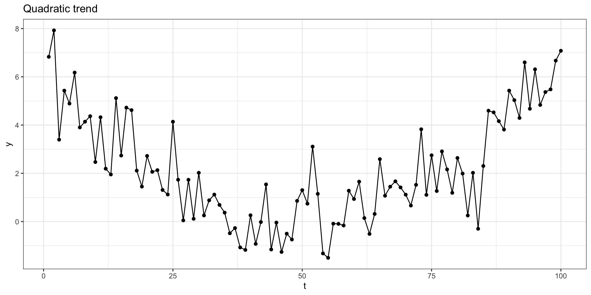
Quadratic trend model

Lets imagine another simple model where \(y_t = \delta + \beta t + \gamma t^2 + x_t\) where \(\delta\), \(\beta\), and \(\gamma\) are constants and \(x_t\) is a stationary process.

Detrending

2nd order differencing

Let \(d_t = y_t - y_{t-1}\) be a first order difference then \(d_t - d_{t-1}\) is a 2nd order difference.

Differencing

Differencing - ACF

AR Models

AR(1)

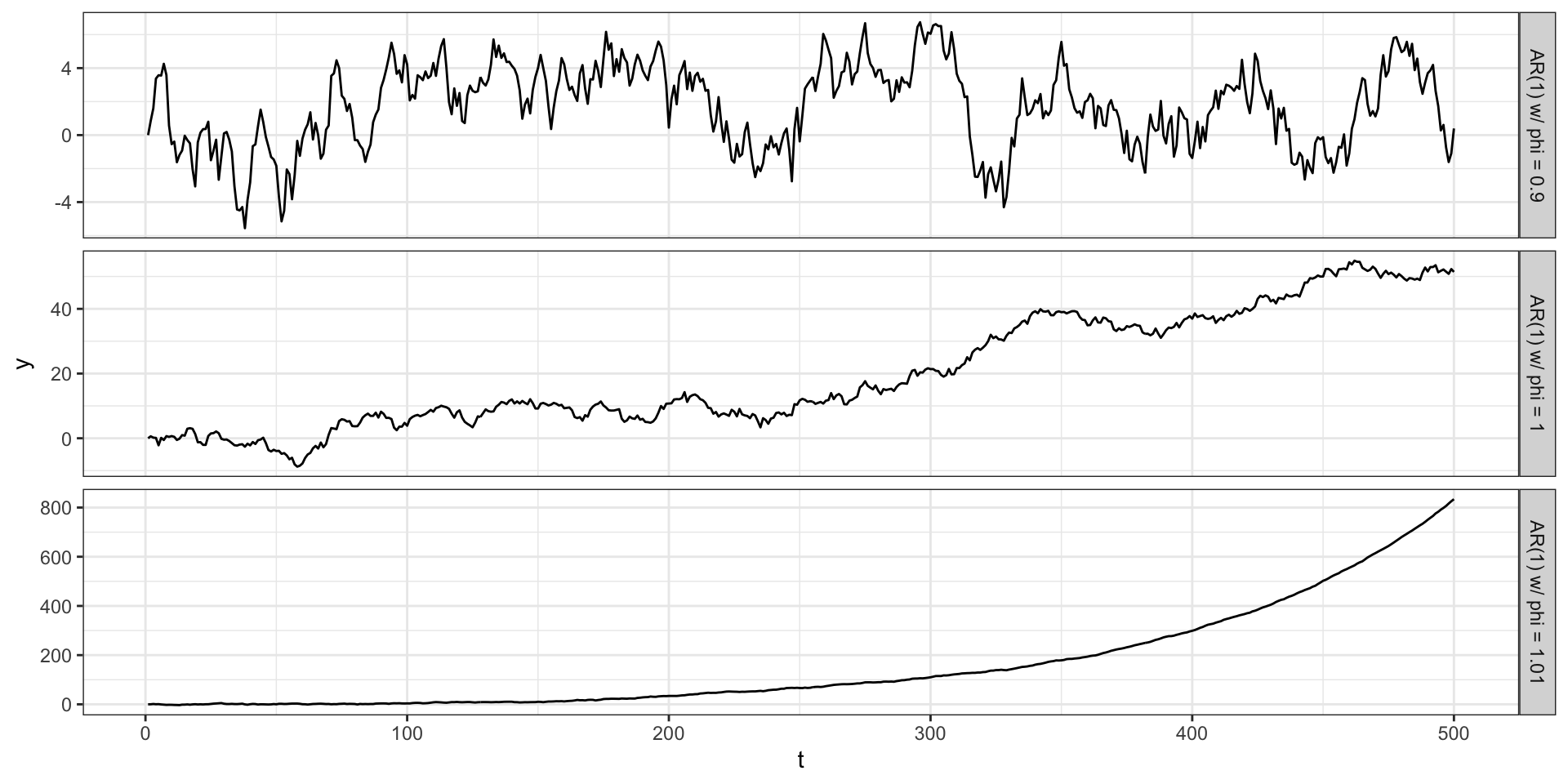
Last time we mentioned a random walk with trend process where \(y_t = \delta + y_{t-1} + w_t\).

The AR(1) process is a generalization of this where we include a coefficient in front of the \(y_{t-1}\) term.

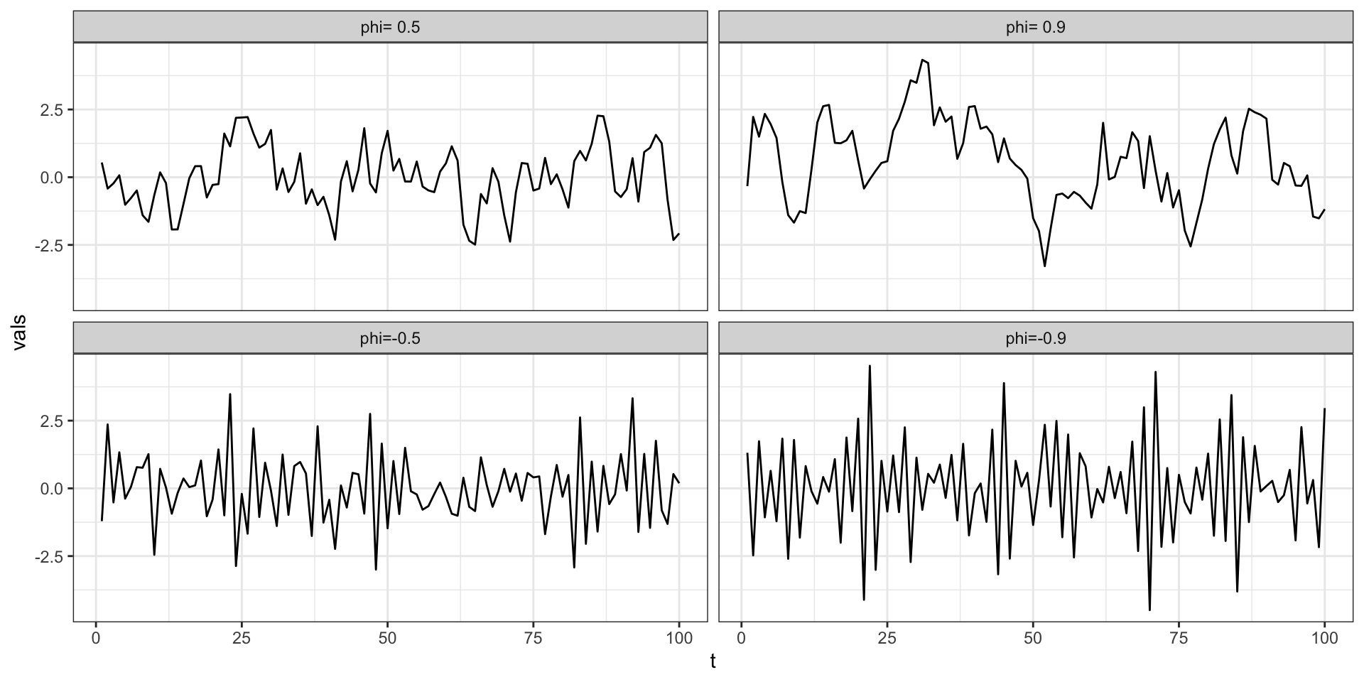
\[AR(1): \quad y_t = \delta + \phi \, y_{t-1} + w_t \] \[ w_t \sim N(0, \sigma^2_w) \]

AR(1) - Positive \(\phi\)

AR(1) - Negative \(\phi\)

Stationarity of \(AR(1)\) processes

Lets rewrite the AR(1) without any autoregressive terms

Stationarity of \(AR(1)\) processes

Under what conditions will an AR(1) process be stationary?

CCFs, Differencing, & AR(1) models

Lagged Predictors and CCFs

Southern Oscillation Index & Recruitment

Time series

Relationship?

`soi` - ACF & PACF

`recruitment` - ACF & PACF

Cross correlation function

Cross correlation function - Scatter plots

Model

Prediction

Residual ACF - Model 3

Autoregessive model 4

Autoregessive model 5

Prediction

Residual ACF - Model 5

Non-stationarity

Non-stationary models

Linear trend model

Differencing

Detrending vs Differencing

Quadratic trend model

Detrending

2nd order differencing

Differencing

Differencing - ACF

AR Models

AR(1)

AR(1) - Positive \(\phi\)

AR(1) - Negative \(\phi\)

Stationarity of \(AR(1)\) processes

Stationarity of \(AR(1)\) processes

Properties of a stationary \(AR(1)\) process

Identifying AR(1) Processes

Identifying AR(1) Processes - ACFs

Identifying AR(1) Processes - PACFs

CCFs, Differencing, & AR(1) models

Lagged Predictors and CCFs

Southern Oscillation Index & Recruitment

Time series

Relationship?

soi - ACF & PACF

recruitment - ACF & PACF

Cross correlation function

Cross correlation function - Scatter plots

Model

Prediction

Residual ACF - Model 3

Autoregessive model 4

Autoregessive model 5

Prediction

Residual ACF - Model 5

Non-stationarity

Non-stationary models

Linear trend model

Differencing

Detrending vs Differencing

Quadratic trend model

Detrending

2nd order differencing

Differencing

Differencing - ACF

AR Models

AR(1)

AR(1) - Positive \(\phi\)

AR(1) - Negative \(\phi\)

Stationarity of \(AR(1)\) processes

Stationarity of \(AR(1)\) processes

Properties of a stationary \(AR(1)\) process

Identifying AR(1) Processes

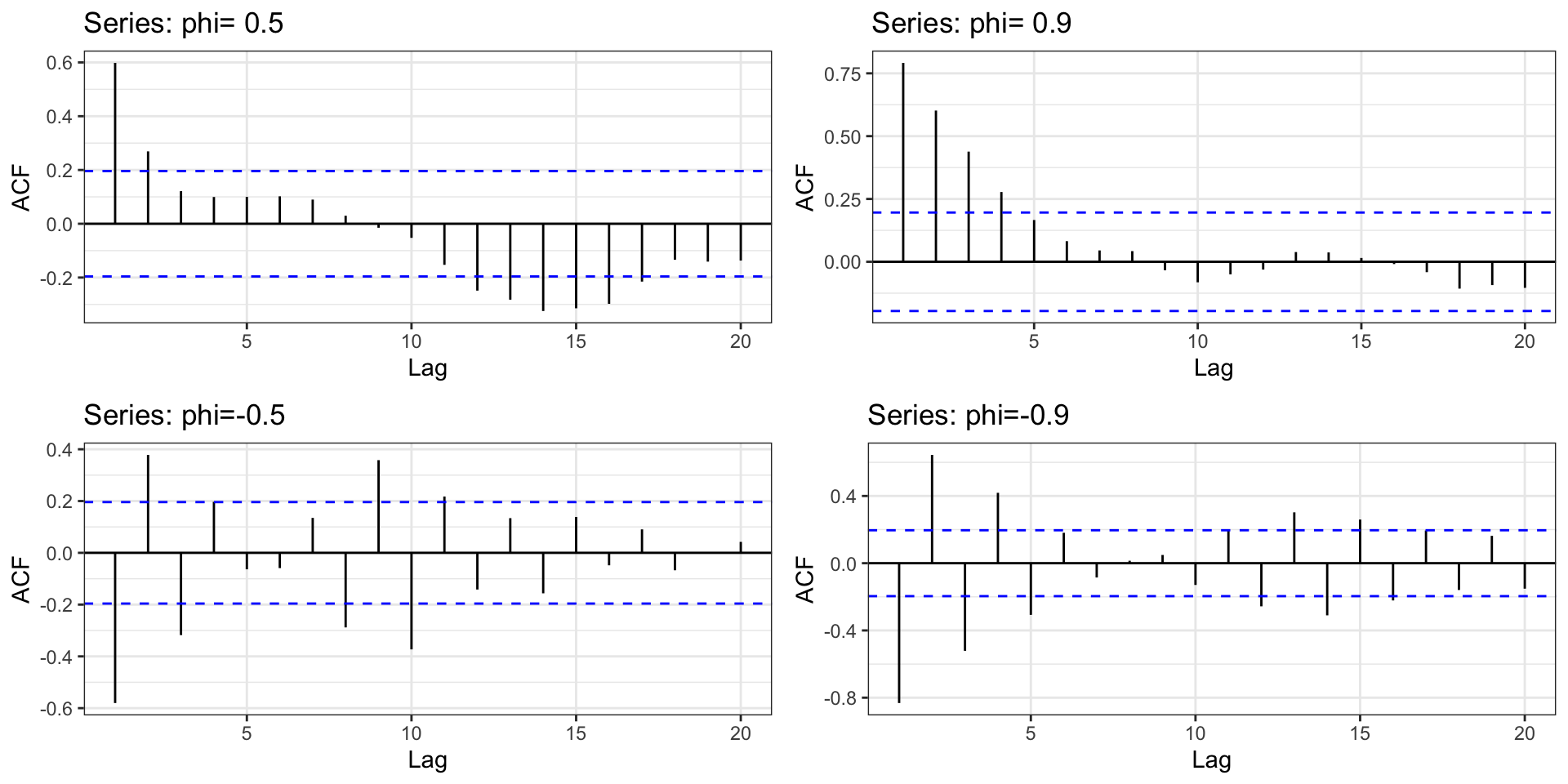
Identifying AR(1) Processes - ACFs

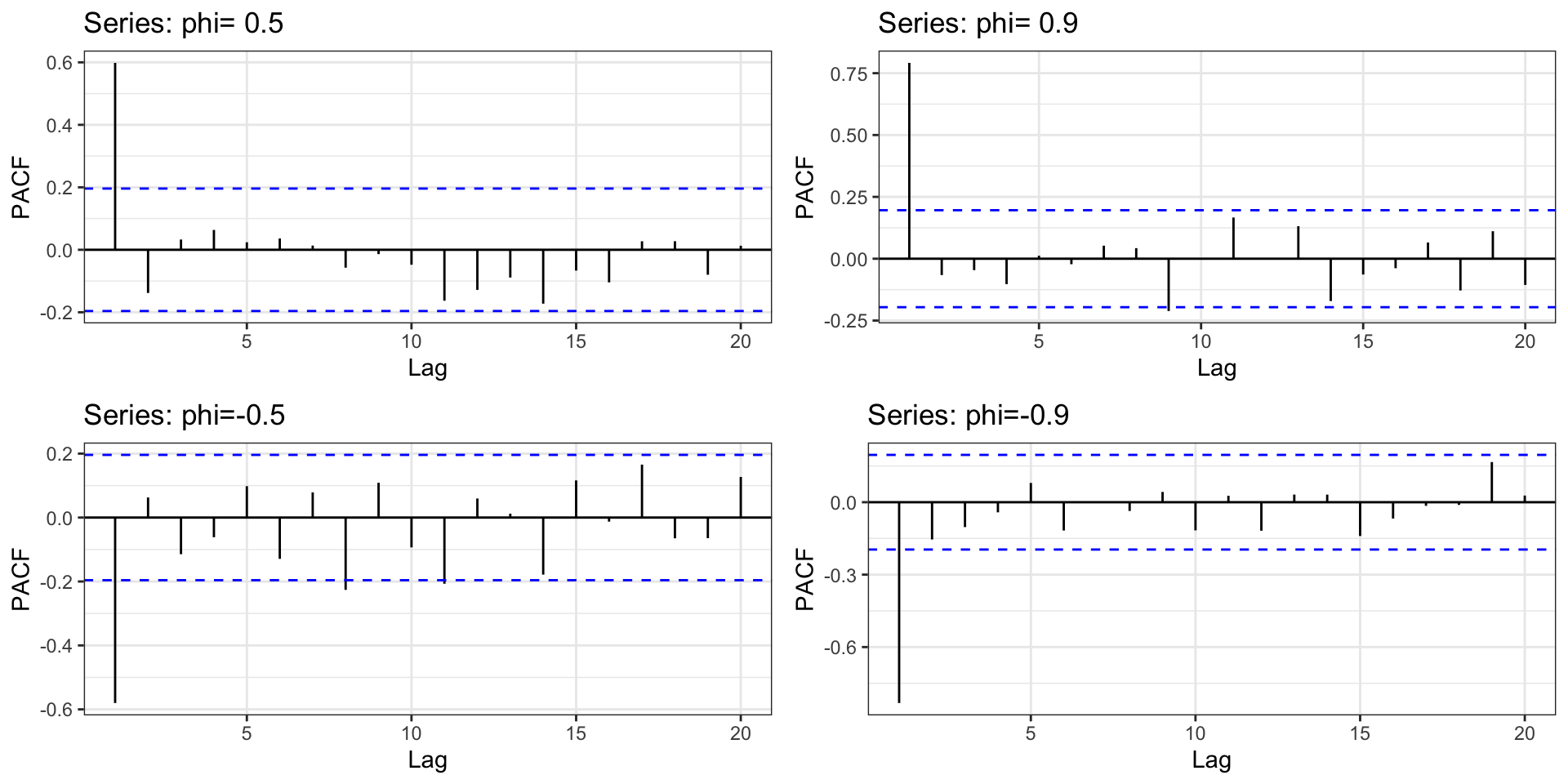
Identifying AR(1) Processes - PACFs

`soi` - ACF & PACF

`recruitment` - ACF & PACF