Logistic Regression and Residual Analysis
Lecture 05
Dr. Colin Rundel
Lecture 4 wrap up
Last time
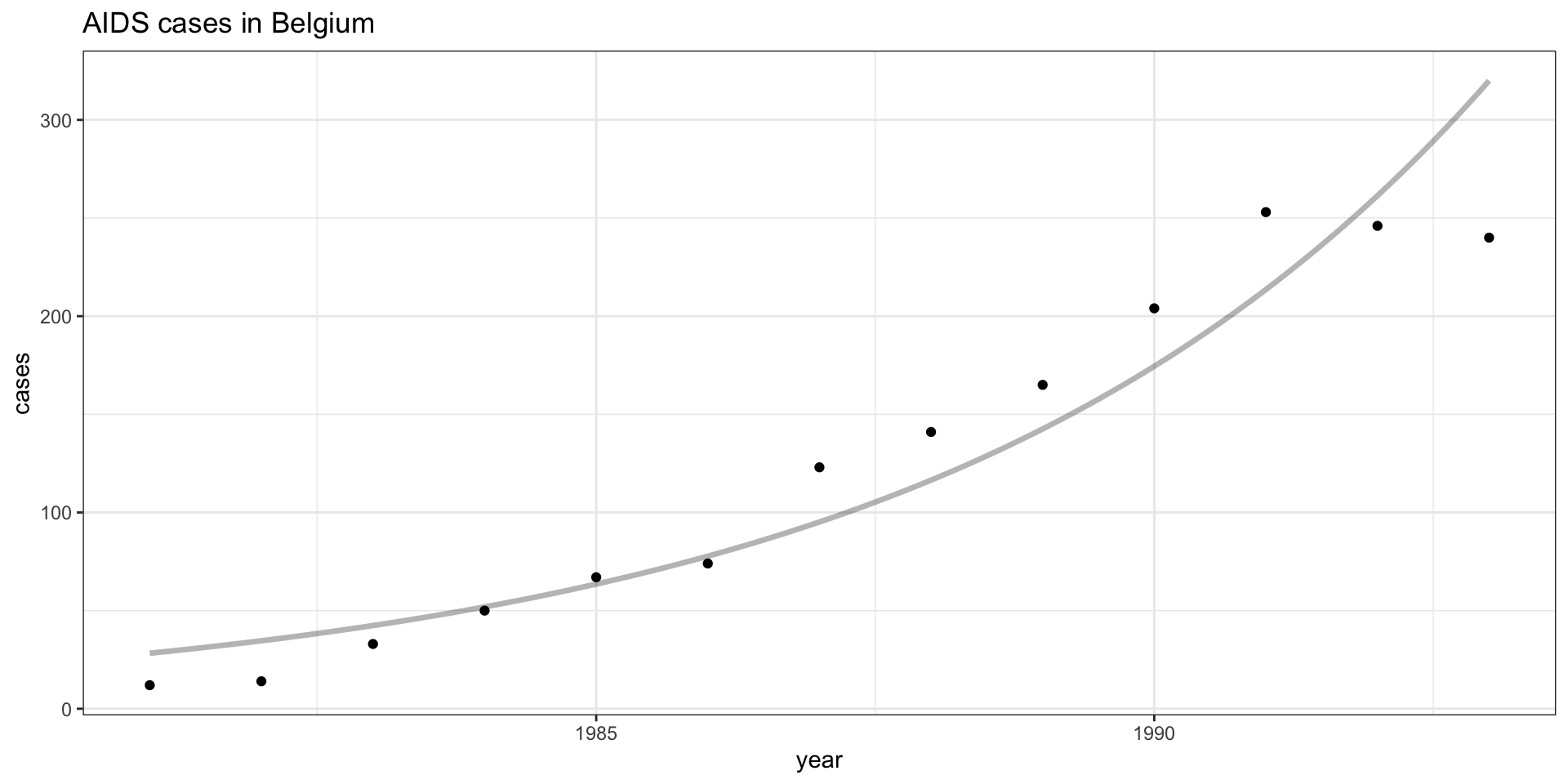
Model Fit
Residuals
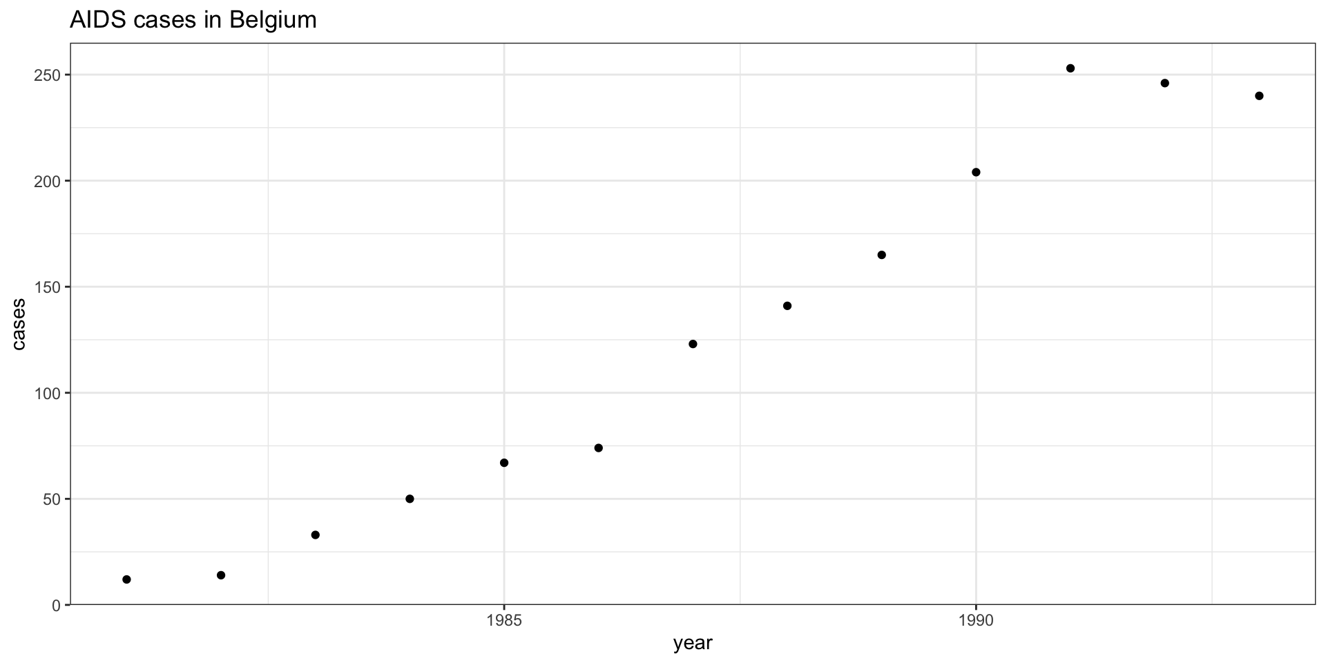
Bayesian Poisson Regression Model
 Family: poisson
  Links: mu = log
Formula: cases ~ year
   Data: aids (Number of observations: 13)
  Draws: 4 chains, each with iter = 2000; warmup = 1000; thin = 1;
         total post-warmup draws = 4000

Population-Level Effects:
          Estimate Est.Error l-95% CI u-95% CI Rhat Bulk_ESS Tail_ESS
Intercept  -397.28     15.38  -427.88  -368.22 1.00     1568     1582
year          0.20      0.01     0.19     0.22 1.00     1569     1582

Draws were sampled using sampling(NUTS). For each parameter, Bulk_ESS
and Tail_ESS are effective sample size measures, and Rhat is the potential
scale reduction factor on split chains (at convergence, Rhat = 1).
Model priors
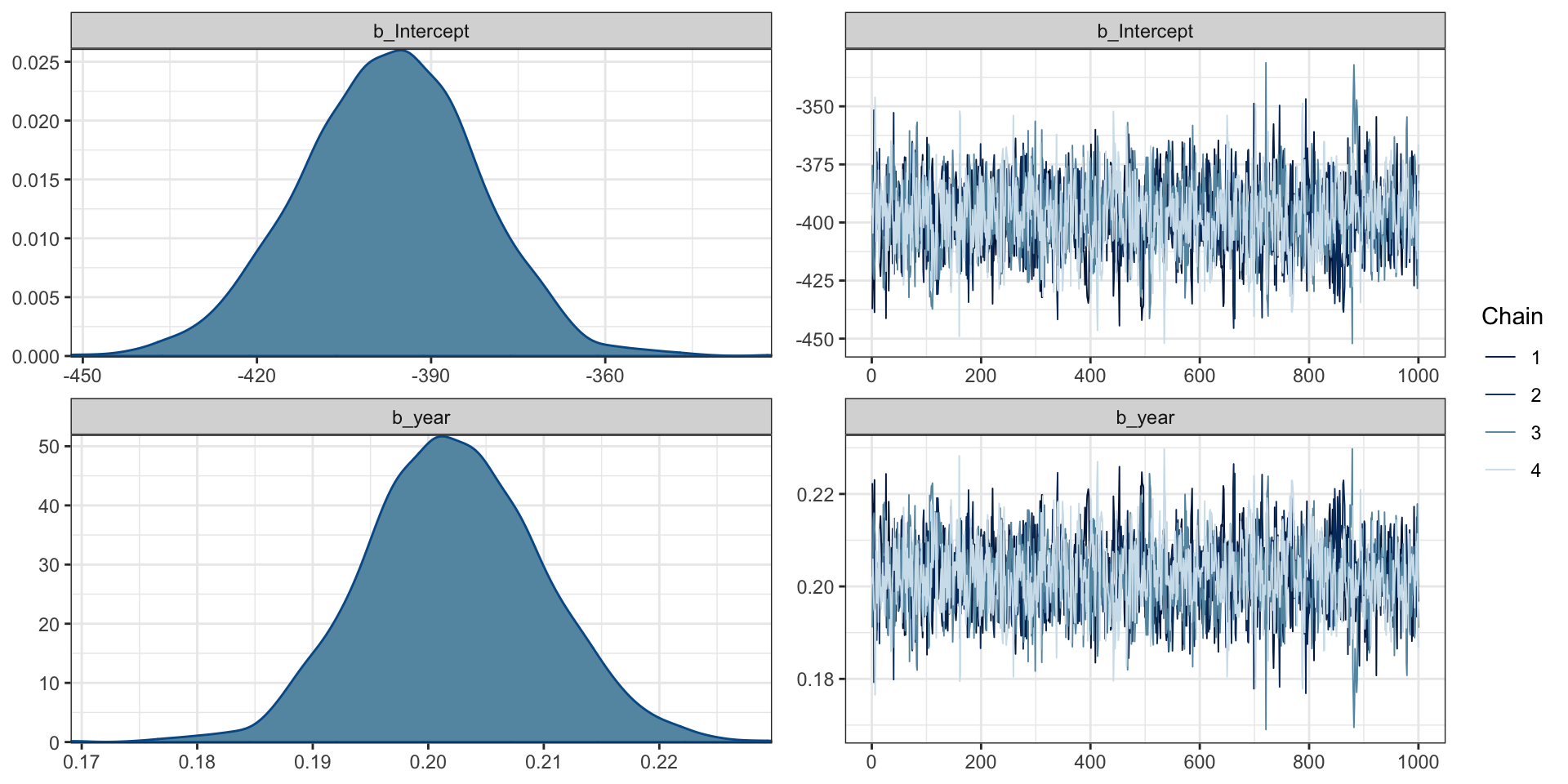
MCMC Diagnostics
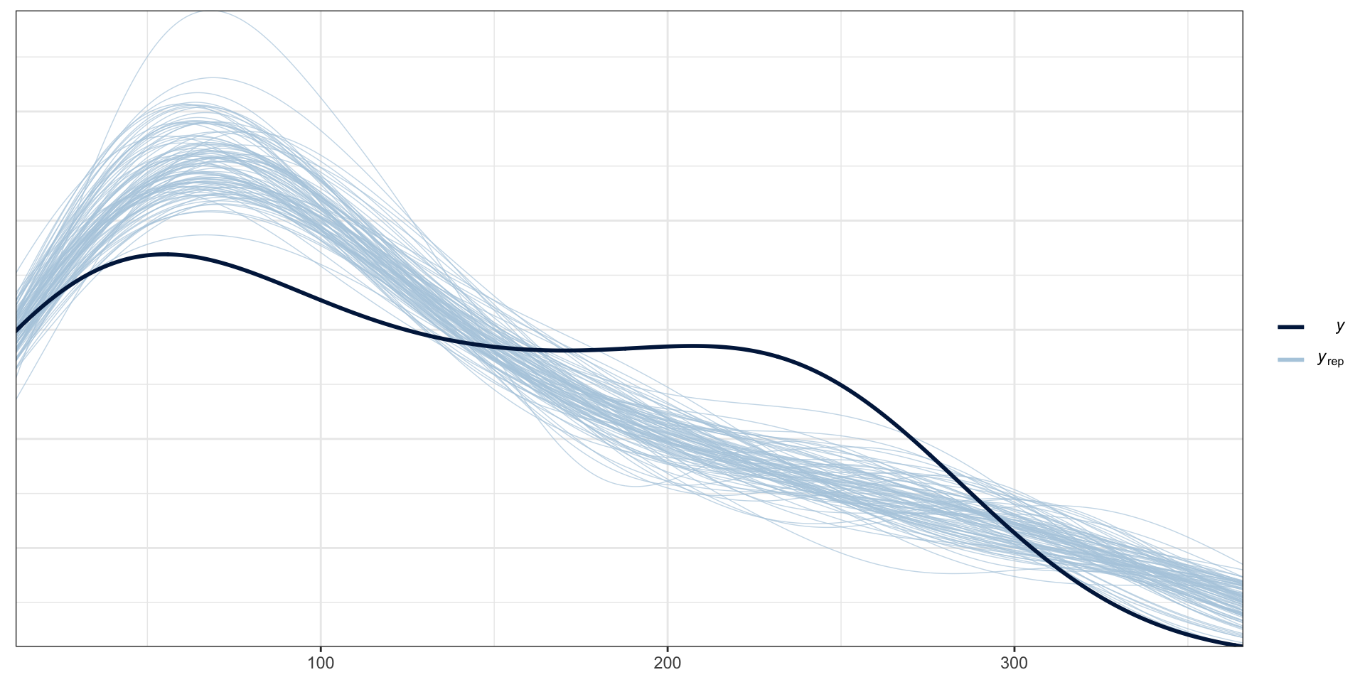
Posterior Predictive Check
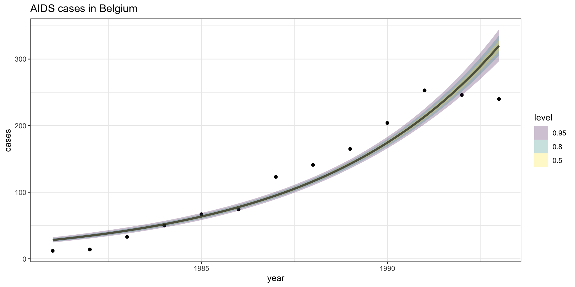
Model fit - \(\lambda\) CI
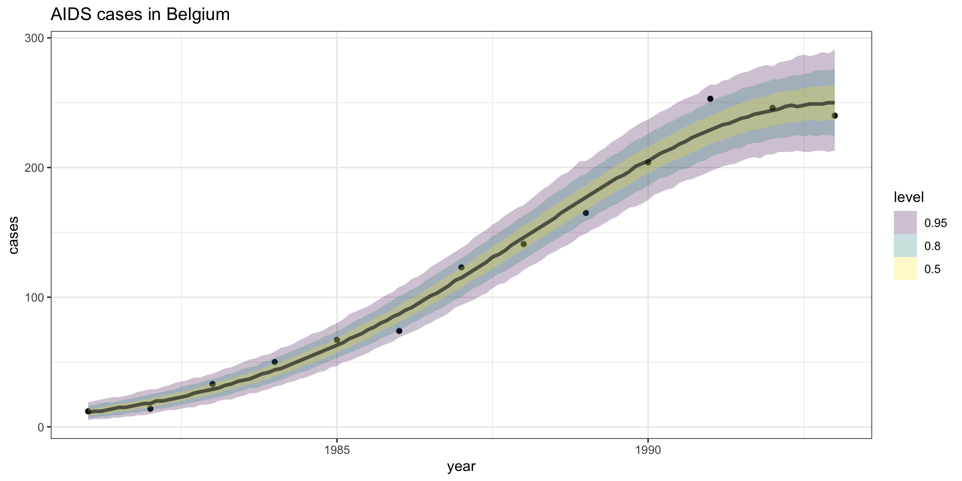
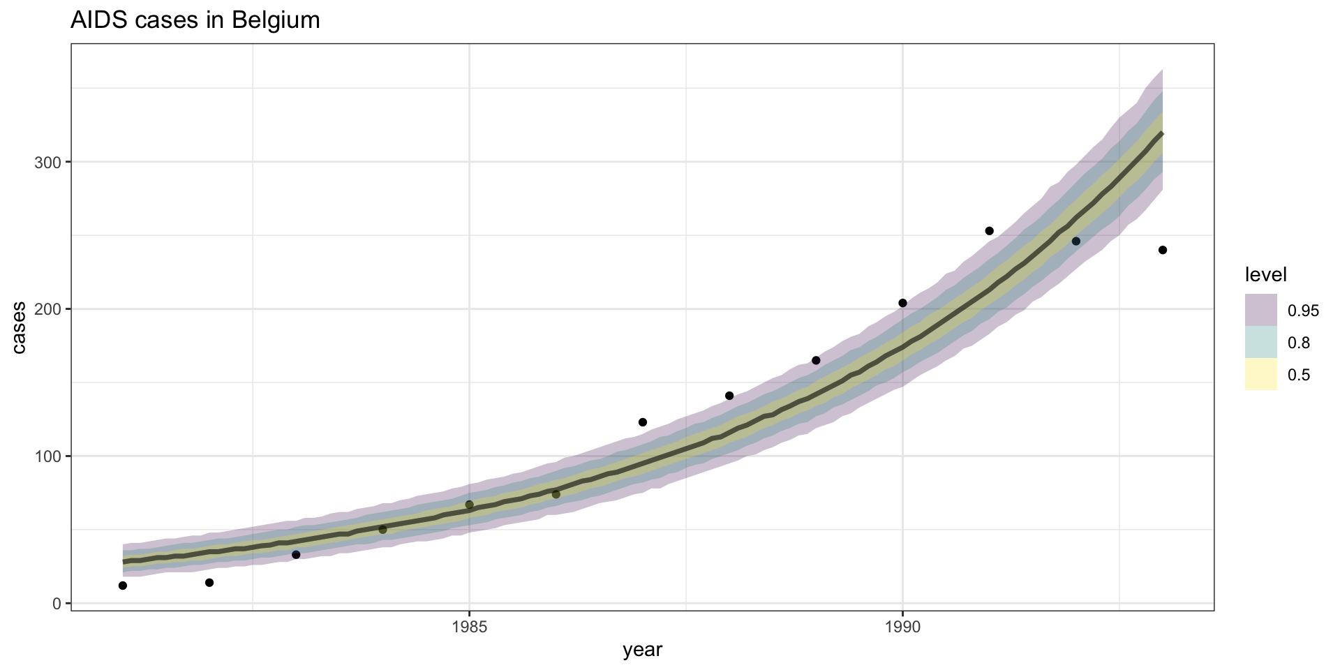
Model fit - \(Y\) CI
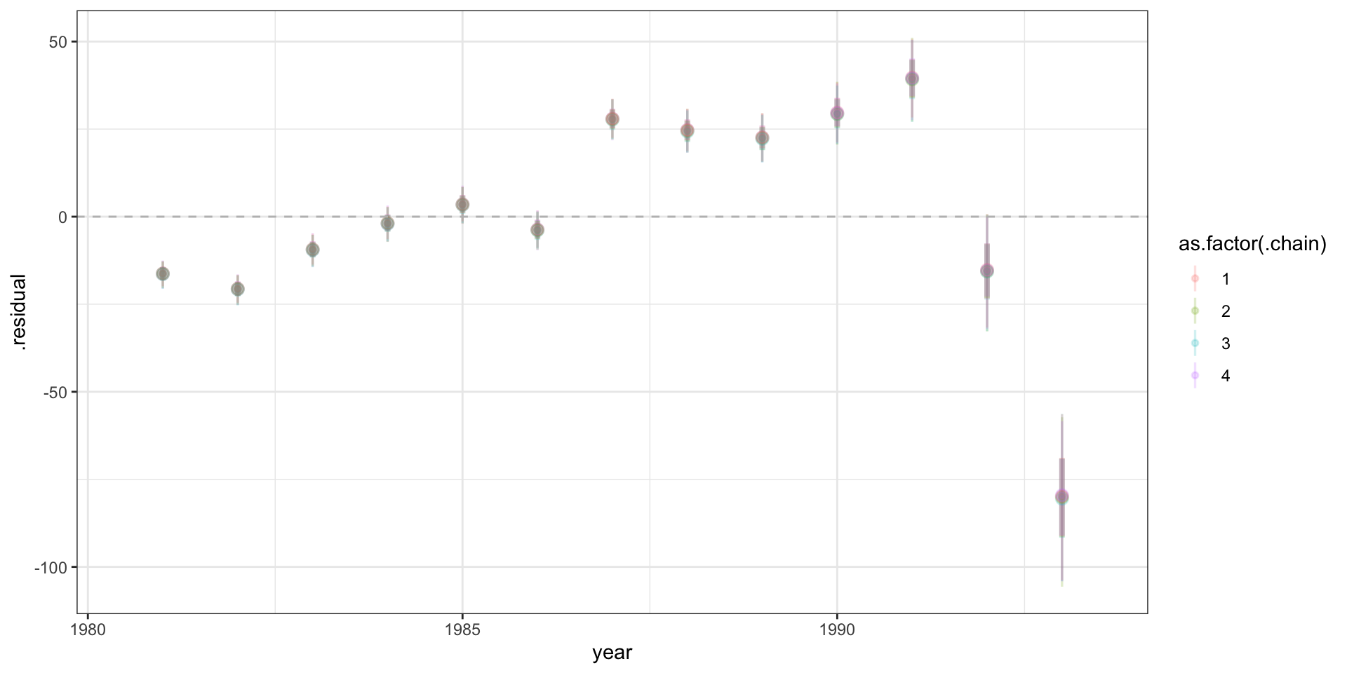
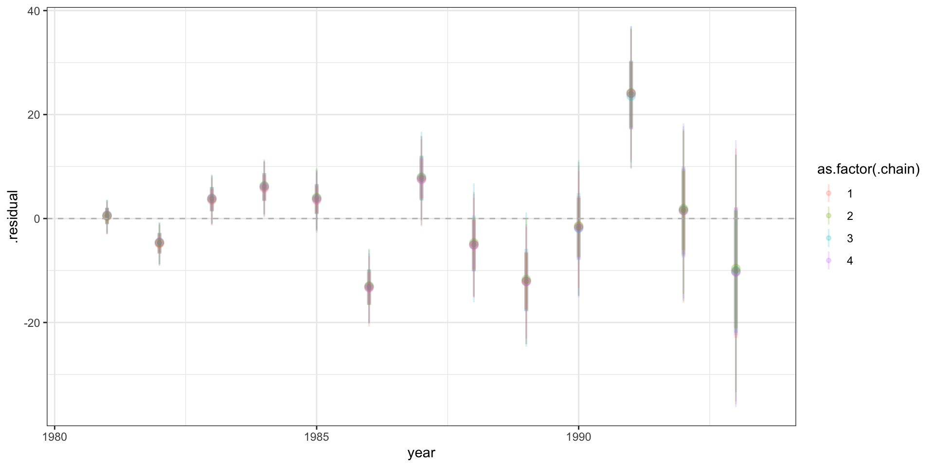
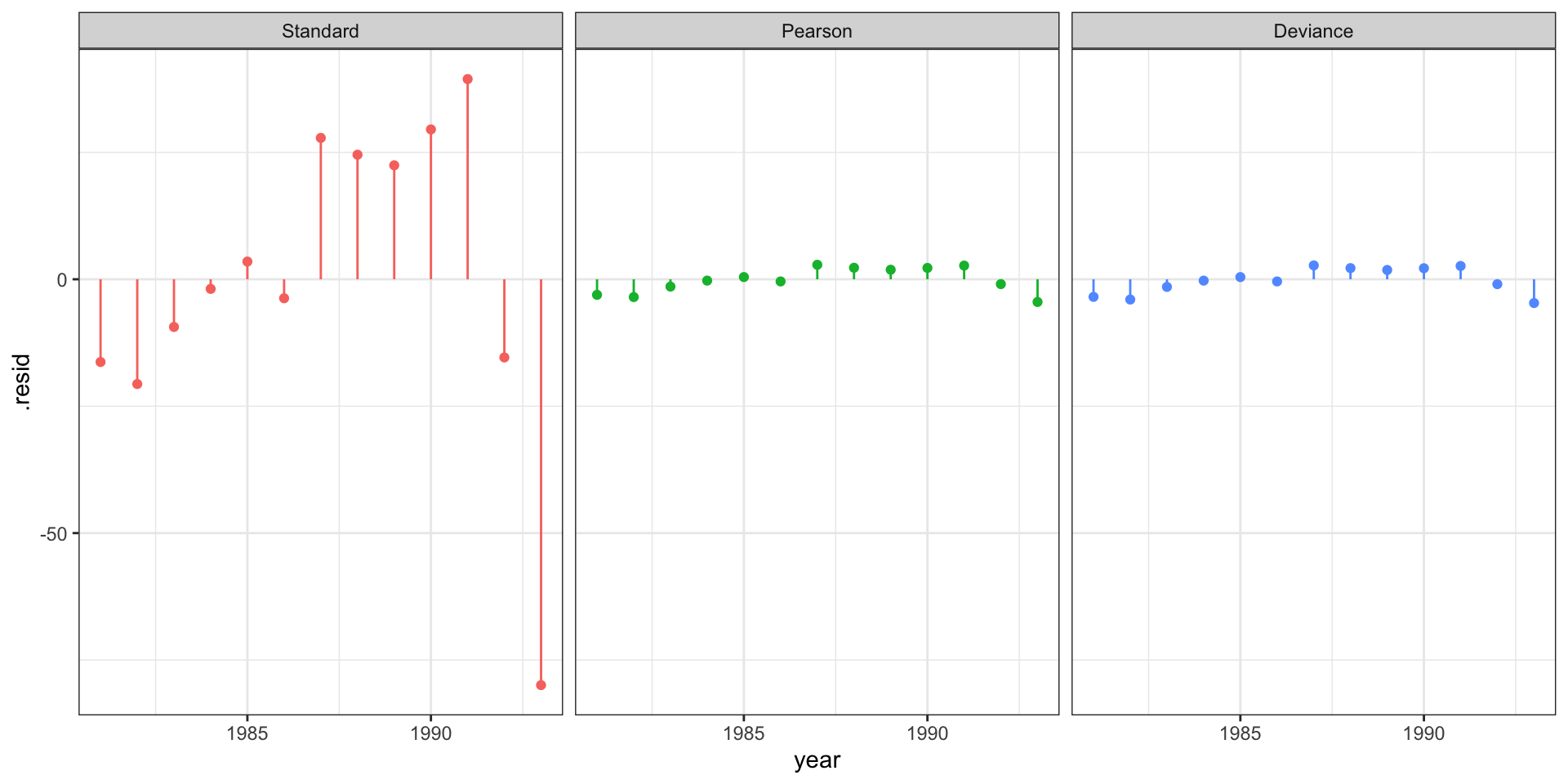
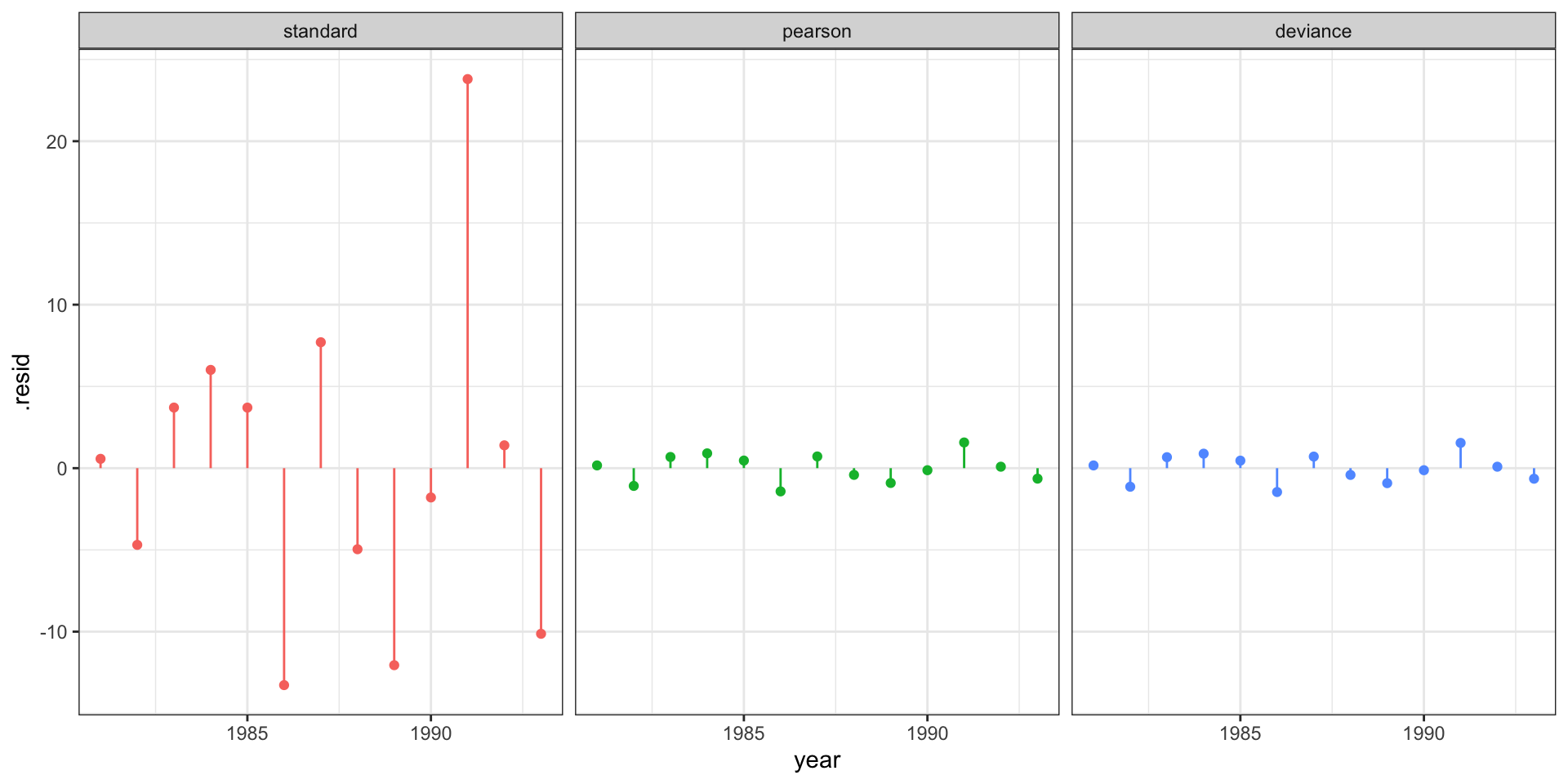
Residuals
# A tibble: 52,000 × 7
    year cases  .row .chain .iteration .draw .residual
   <int> <int> <int>  <int>      <int> <int>     <dbl>
 1  1981    12     1      1          1     1     -11.4
 2  1981    12     1      1          2     2     -14.0
 3  1981    12     1      1          3     3     -13.1
 4  1981    12     1      1          4     4     -12.2
 5  1981    12     1      1          5     5     -12.0
 6  1981    12     1      1          6     6     -19.8
 7  1981    12     1      1          7     7     -18.7
 8  1981    12     1      1          8     8     -18.7
 9  1981    12     1      1          9     9     -20.3
10  1981    12     1      1         10    10     -19.5
# … with 51,990 more rows
Residual plot
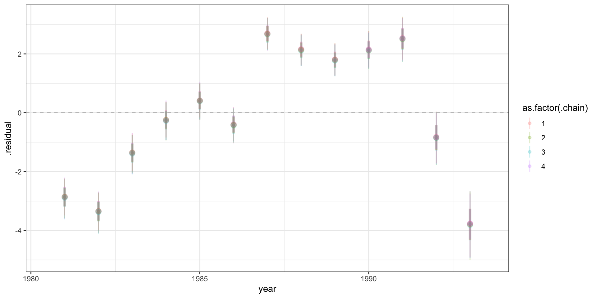
Standardized residuals?
Model performance - rmse, crps
predicted_draws_fix(g_bayes, newdata = aids) |>
  group_by(.chain, .row) |>
  summarize(
    rmse = yardstick::rmse_vec(cases, .prediction),
    crps = calc_crps(.prediction, cases)
  ) |>
  group_by(.chain) |>
  summarize(
    rmse = mean(rmse),
    crps = mean(crps)
  )
# A tibble: 4 × 3
.chain rmse crps
<int> <dbl> <dbl>
1 1 26.3 17.7
2 2 26.1 17.5
3 3 26.3 17.7
4 4 26.3 17.8Model performance - emp coverage
predicted_draws_fix(g_bayes, newdata = aids) |>
  group_by(.row, cases) |>
  tidybayes::mean_hdi(
    .prediction, .width = c(0.5,0.9,0.95)
  ) |>
  mutate(contains = cases >= .lower & cases <= .upper) %>%
  group_by(.width) |>
  summarize(
    emp_cov = sum(contains)/n()
  )
# A tibble: 3 × 2
.width emp_cov
<dbl> <dbl>
1 0.5 0.154
2 0.9 0.385
3 0.95 0.462Updating the model
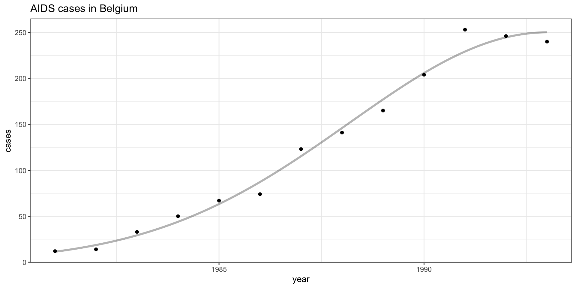
Quadratic fit
Quadratic fit - residuals
Bayesian quadratic fit
 Family: poisson
  Links: mu = log
Formula: cases ~ year + I(year^2)
   Data: aids (Number of observations: 13)
  Draws: 4 chains, each with iter = 2000; warmup = 1000; thin = 1;
         total post-warmup draws = 4000

Population-Level Effects:
          Estimate Est.Error  l-95% CI u-95% CI Rhat Bulk_ESS Tail_ESS
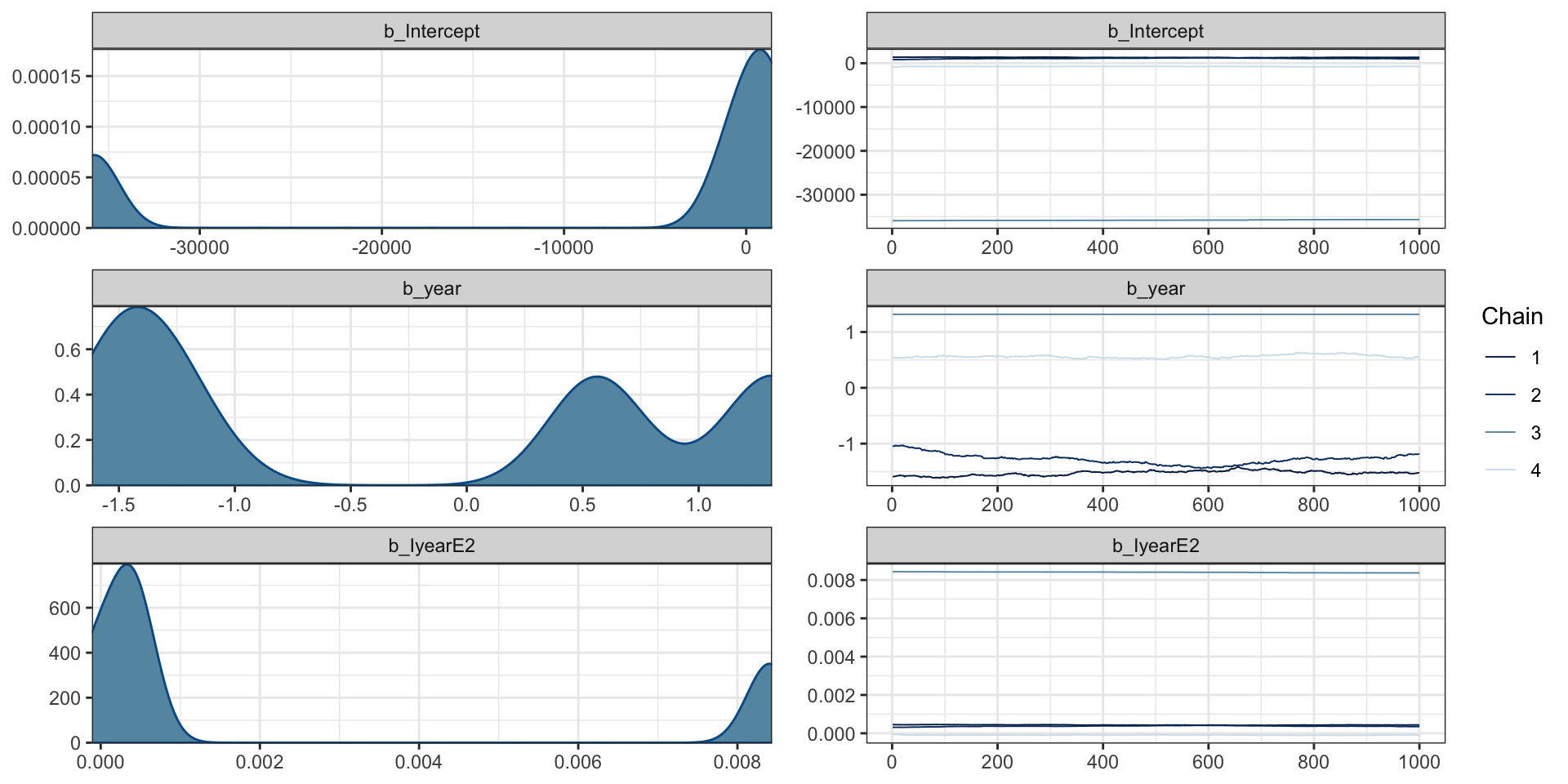
Intercept -8538.33  15758.51 -35873.48  1378.93 3.72        4       11
year         -0.23      1.21     -1.59     1.32 3.73        4       11
IyearE2       0.00      0.00     -0.00     0.01 3.56        4       11

Draws were sampled using sampling(NUTS). For each parameter, Bulk_ESS
and Tail_ESS are effective sample size measures, and Rhat is the potential
scale reduction factor on split chains (at convergence, Rhat = 1).
Diagnostics
Bayesian quadratic fit (fixed)
 Family: poisson
  Links: mu = log
Formula: cases ~ I(year - min(year)) + I((year - min(year))^2)
   Data: aids (Number of observations: 13)
  Draws: 4 chains, each with iter = 2000; warmup = 1000; thin = 1;
         total post-warmup draws = 4000

Population-Level Effects:
                Estimate Est.Error l-95% CI u-95% CI Rhat Bulk_ESS Tail_ESS
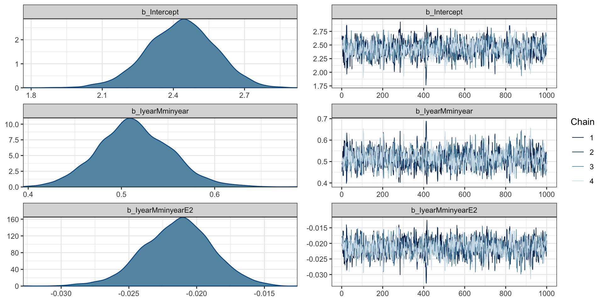
Intercept           2.43      0.14     2.14     2.70 1.00     1012     1259
IyearMminyear       0.51      0.04     0.44     0.59 1.00     1079     1342
IyearMminyearE2    -0.02      0.00    -0.03    -0.02 1.00     1180     1408

Draws were sampled using sampling(NUTS). For each parameter, Bulk_ESS
and Tail_ESS are effective sample size measures, and Rhat is the potential
scale reduction factor on split chains (at convergence, Rhat = 1).
Diagnostics
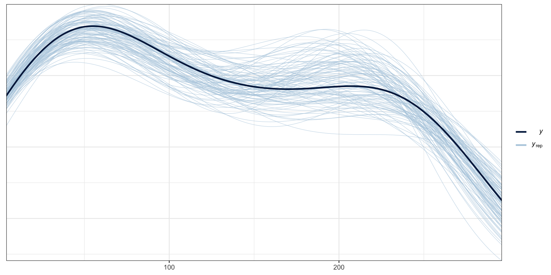
PP Checks
Model fit - \(Y\) CI
Residuals
Model performance - rmse, crps
predicted_draws_fix(g2_bayes, newdata = aids) |>
  group_by(.chain, .row) |>
  summarize(
    rmse = yardstick::rmse_vec(cases, .prediction),
    crps = calc_crps(.prediction, cases)
  ) |>
  group_by(.chain) |>
  summarize(
    rmse = mean(rmse),
    crps = mean(crps)
  )
# A tibble: 4 × 3
.chain rmse crps
<int> <dbl> <dbl>
1 1 14.1 5.19
2 2 14.2 5.06
3 3 14.2 5.09
4 4 14.2 4.99Model performance - emp coverage
predicted_draws_fix(g2_bayes, newdata = aids) |>
  group_by(.row, cases) |>
  tidybayes::mean_hdi(
    .prediction, .width = c(0.5,0.9,0.95)
  ) |>
  mutate(contains = cases >= .lower & cases <= .upper) %>%
  group_by(.width) |>
  summarize(
    emp_cov = sum(contains)/n()
  )
# A tibble: 3 × 2
.width emp_cov
<dbl> <dbl>
1 0.5 0.692
2 0.9 1
3 0.95 1 Logistic regression
Logistic regression as a GLM
This is another case of a generalized linear model, specifically where the outcome is 0-1 data (i.e. Bernoulli draws),
\[ \begin{aligned} Y_i &\sim \text{Bern}(p_i)\\ \text{logit} \, E(Y_i|\boldsymbol{X}_{i\cdot}) &= \text{logit}(p_i) = \underset{1 \times p}{\boldsymbol{X}_{i\cdot}}\underset{p \times 1}{\boldsymbol{\beta}} \\ \\ E(Y_i) &= p_i \\ Var(Y_i) &= p_i(1-p_i) \\ \\ \text{logit}(p_i) &= \log \frac{p_i}{1-p_i} \\ \text{logit}^{-1}(x) &= \frac{\exp(x)}{1+\exp(x)} = \frac{1}{1+\exp(-x)} \end{aligned} \]
Background
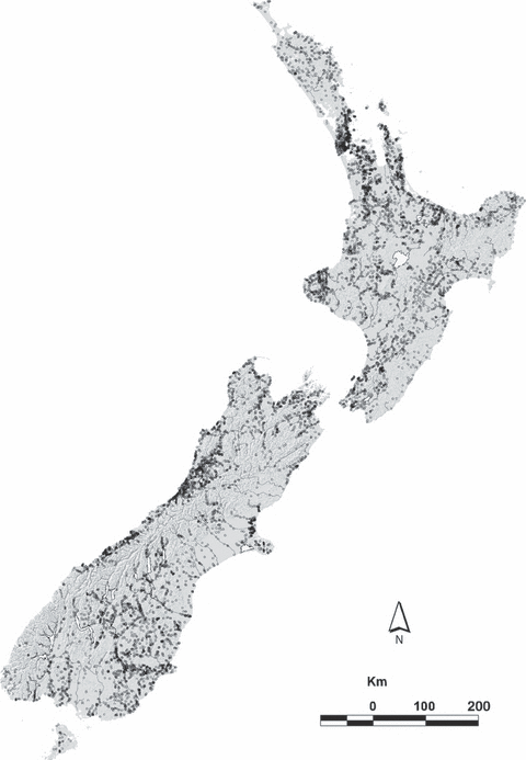
Next we’ll be looking at data on the presence and absence of the short-finned eel (Anguilla australis) at a number of sites in New Zealand.
These data come from
- Leathwick, J. R., Elith, J., Chadderton, W. L., Rowe, D. and Hastie, T. (2008), Dispersal, disturbance and the contrasting biogeographies of New Zealand’s diadromous and non-diadromous fish species. Journal of Biogeography, 35: 1481–1497.

Species Distribution
Codebook:
presence- presence (1) or absence (0) of Anguilla australis at the sampling locationSegSumT- Summer air temperature (degrees C)DSDist- Distance to coast (km)DSMaxSlope- Maximum downstream slope (degrees)USRainDays- days per month with rain greater than 25 mmUSSlope- average slope in the upstream catchment (degrees)USNative- area with indigenous forest (proportion)DSDam- Presence of known downstream obstructions, mostly damsMethod- fishing method (electric,net,spot,trap, ormixture)LocSed- weighted average of proportional cover of bed sediment- mud
- sand
- fine gravel
- coarse gravel
- cobble
- boulder
- bedrock
Data
# A tibble: 824 × 10
presence SegSumT DSDist DSMaxSl…¹ USRai…² USSlope USNat…³ DSDam Method LocSed
<int> <dbl> <dbl> <dbl> <dbl> <dbl> <dbl> <int> <fct> <dbl>
1 0 16 50.2 0.57 2.47 9.8 0.81 0 elect… 4.8
2 1 18.7 133. 1.15 1.15 8.3 0.34 0 elect… 2
3 0 18.3 107. 0.57 0.847 0.4 0 0 spo 1
4 0 16.7 167. 1.72 0.21 0.4 0.22 1 elect… 4
5 1 17.2 3.95 1.15 1.98 21.9 0.96 0 elect… 4.7
6 0 15.1 11.2 1.72 3.3 25.7 1 0 elect… 4.5
7 0 12.7 42.4 2.86 0.43 9.6 0.09 0 elect… 4.3
8 1 18.2 94.4 3.43 0.847 20.5 0.92 0 elect… 3.6
9 0 14.9 45.7 2.29 2.25 3.9 0.38 0 elect… 3.7
10 1 18.3 91.9 1.72 0.861 6.7 0.58 1 elect… 1
# … with 814 more rows, and abbreviated variable names ¹DSMaxSlope,
# ²USRainDays, ³USNativeTest / train split
EDA
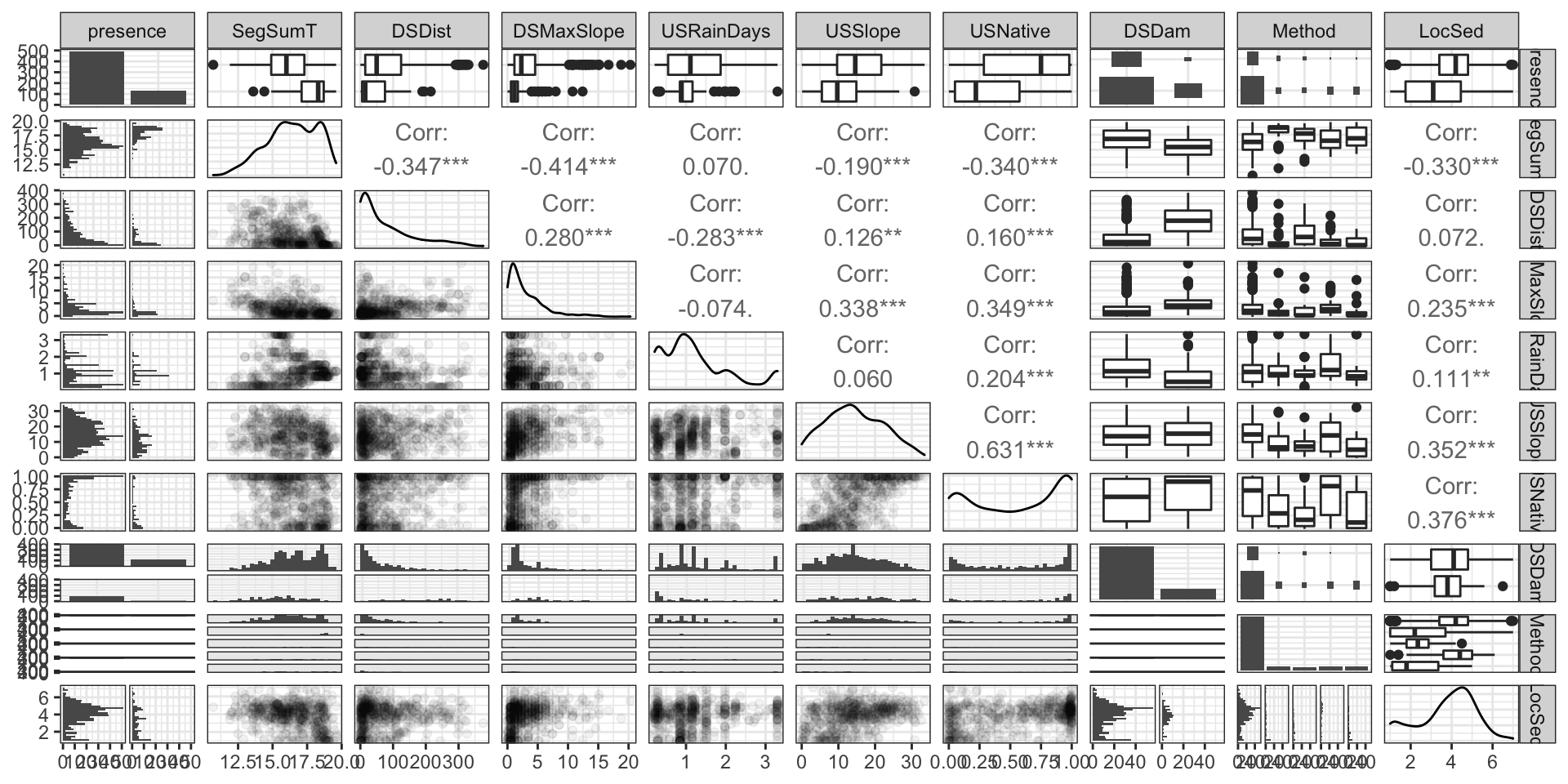
EDA (part 1)
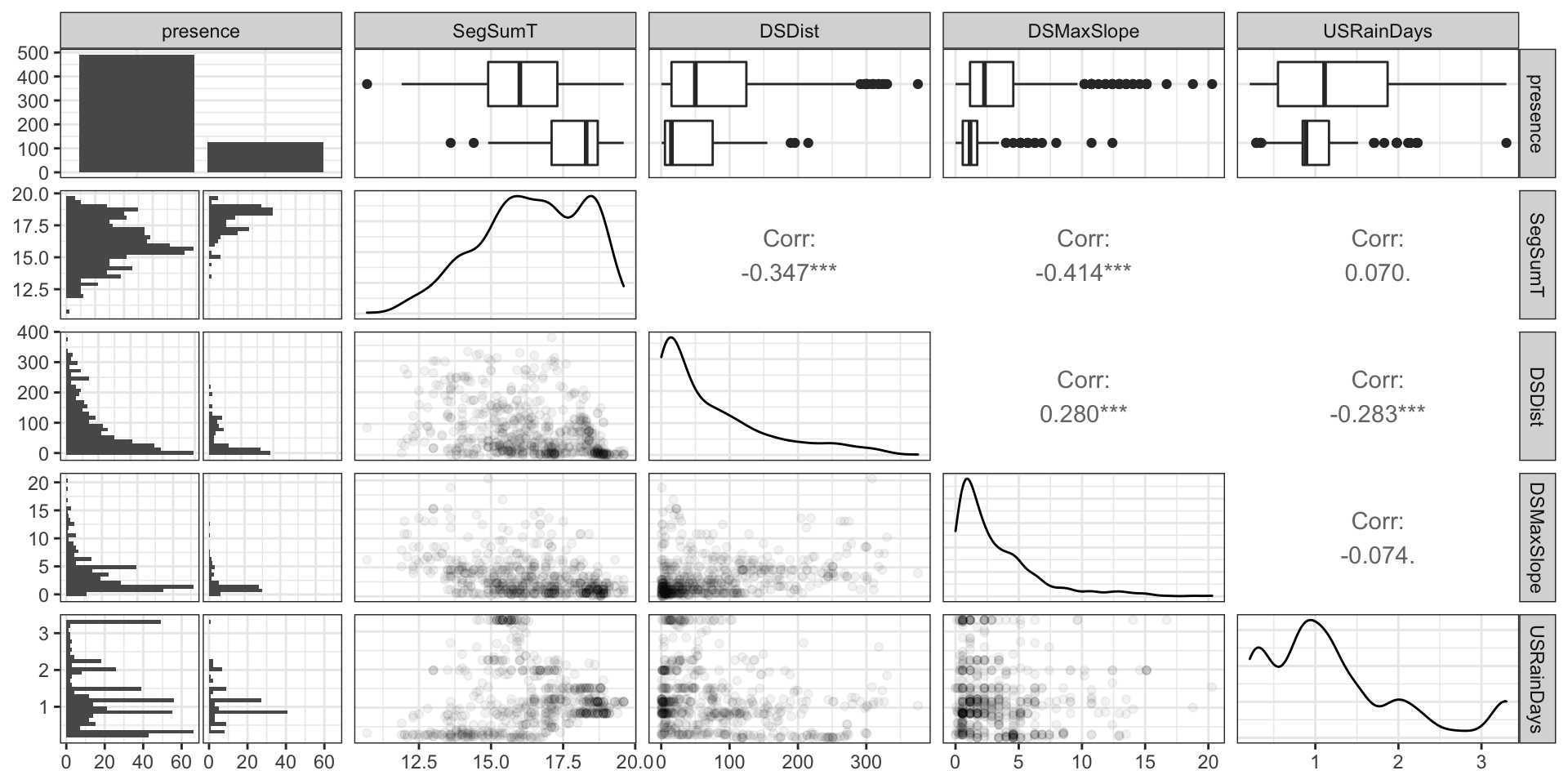
EDA (part 2)
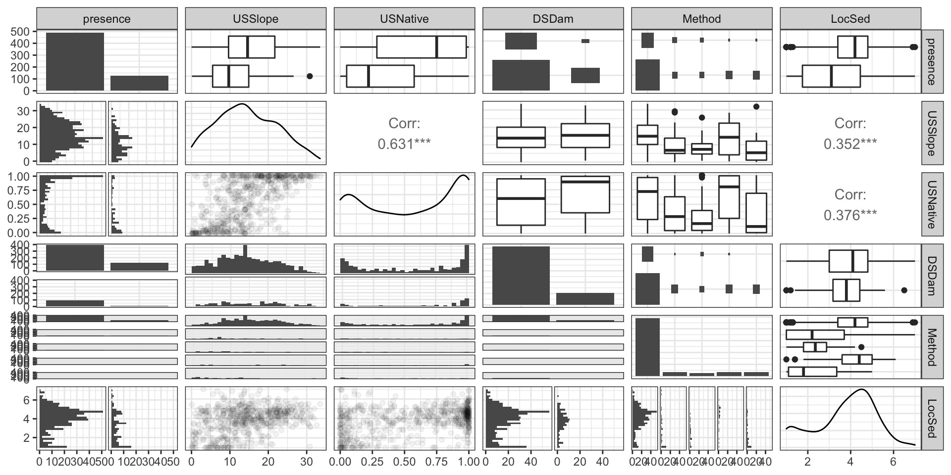
EDA (part 3)
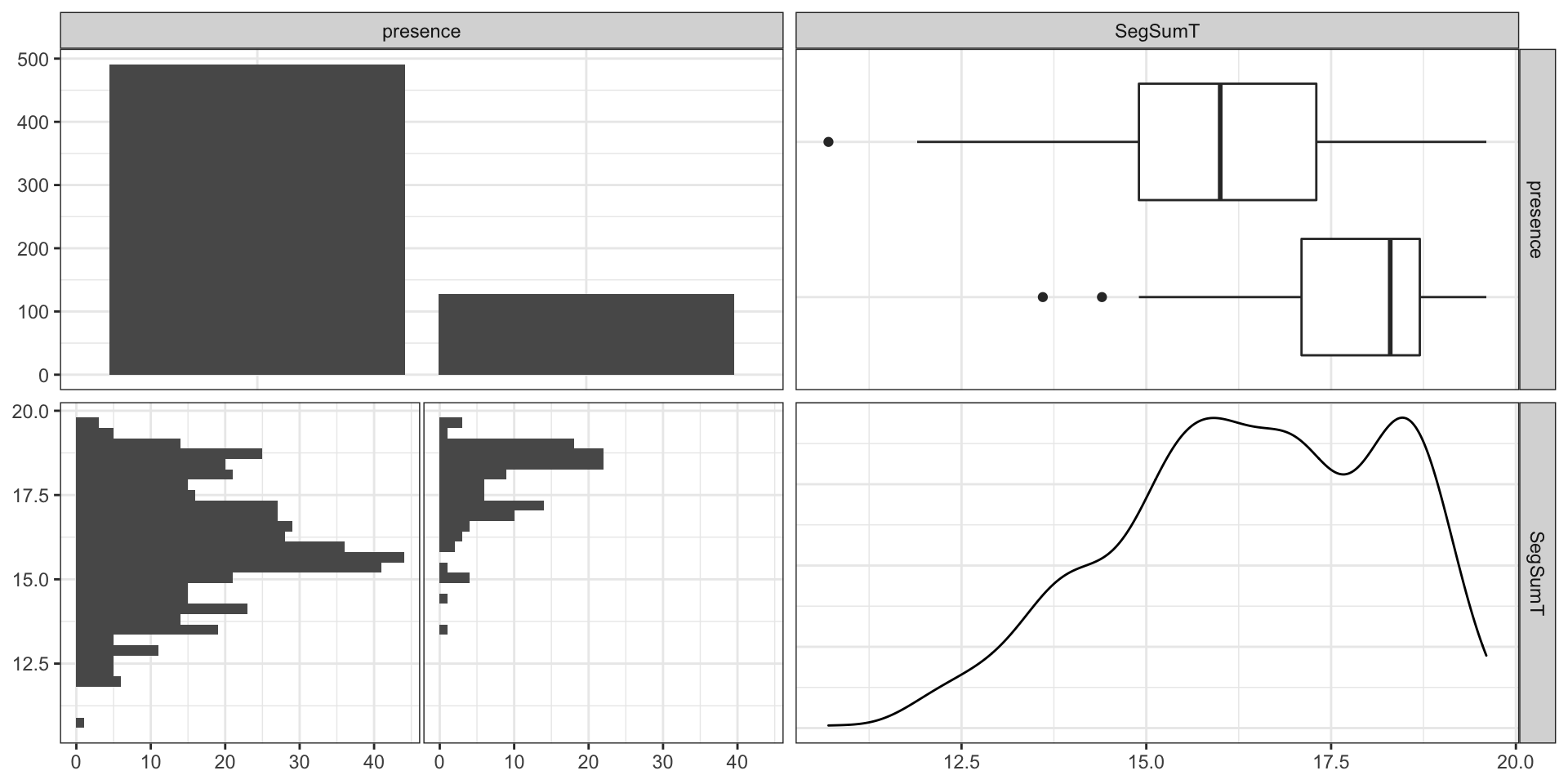
Basic Model
Model
Call:
glm(formula = presence ~ SegSumT, family = binomial, data = anguilla_train)

Deviance Residuals:
    Min       1Q   Median       3Q      Max
-1.4707  -0.6598  -0.3759  -0.1417   2.8815

Coefficients:
             Estimate Std. Error z value Pr(>|z|)
(Intercept) -15.02201    1.53770  -9.769   <2e-16 ***
SegSumT       0.80047    0.08726   9.173   <2e-16 ***
---
Signif. codes:  0 '***' 0.001 '**' 0.01 '*' 0.05 '.' 0.1 ' ' 1

(Dispersion parameter for binomial family taken to be 1)

    Null deviance: 627.81  on 617  degrees of freedom
Residual deviance: 501.93  on 616  degrees of freedom
AIC: 505.93

Number of Fisher Scoring iterations: 5
Fit
# A tibble: 618 × 8
   presence SegSumT .fitted .resid .std.resid    .hat .sigma   .cooksd
      <int>   <dbl>   <dbl>  <dbl>      <dbl>   <dbl>  <dbl>     <dbl>
 1        0    16.4  0.131  -0.529     -0.530 0.00260  0.903 0.000197
 2        1    17.1  0.209   1.77       1.77  0.00232  0.901 0.00443
 3        0    14    0.0216 -0.209     -0.209 0.00231  0.903 0.0000256
 4        0    18.2  0.389  -0.992     -0.994 0.00364  0.903 0.00117
 5        0    15.6  0.0735 -0.391     -0.391 0.00286  0.903 0.000114
 6        0    18.3  0.408  -1.02      -1.03  0.00395  0.902 0.00137
 7        0    18.5  0.447  -1.09      -1.09  0.00466  0.902 0.00190
 8        0    16.2  0.114  -0.491     -0.492 0.00270  0.903 0.000174
 9        0    18    0.351  -0.930     -0.932 0.00313  0.903 0.000853
10        1    17.3  0.236   1.70       1.70  0.00233  0.901 0.00379
# … with 608 more rows
Visually
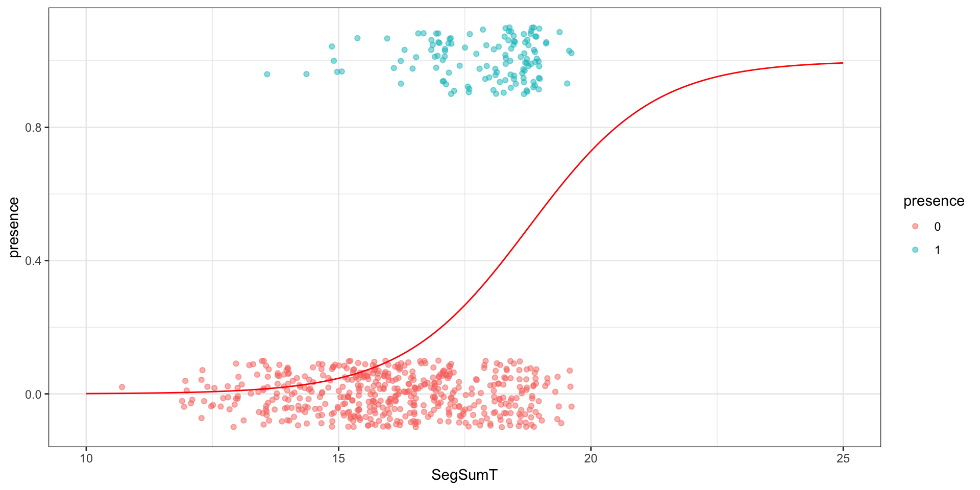
Separation
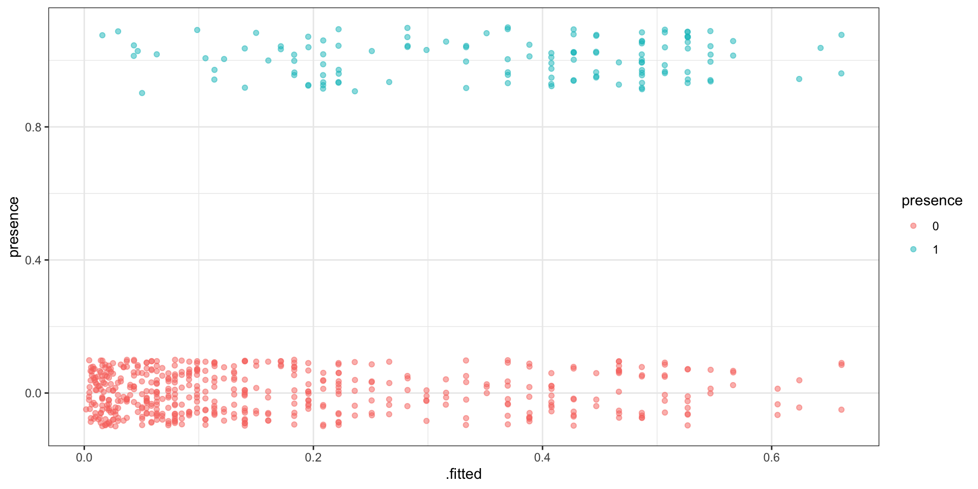
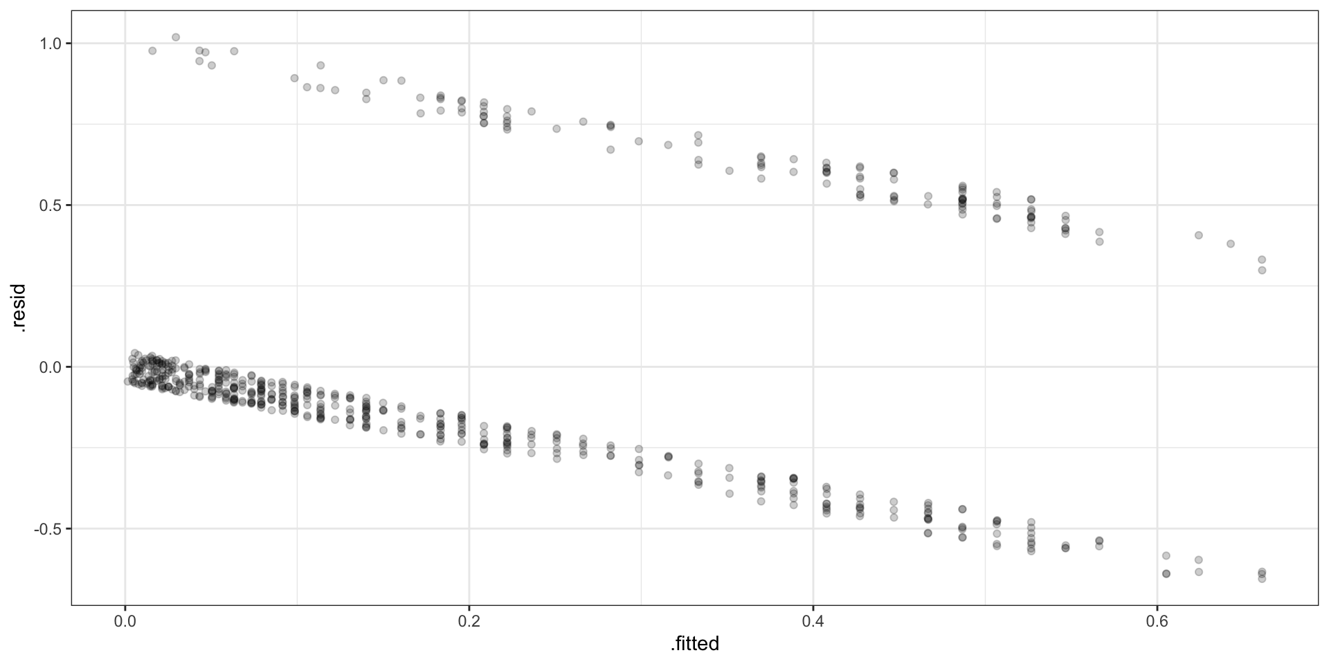
Standard Residuals
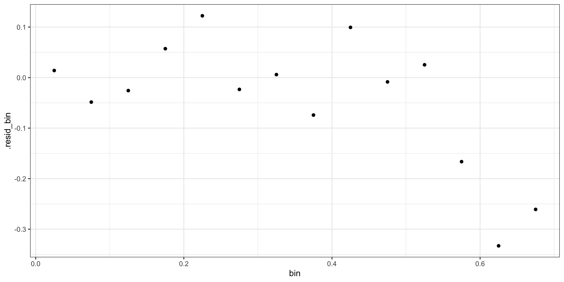
Binned Residuals
Pearson Residuals
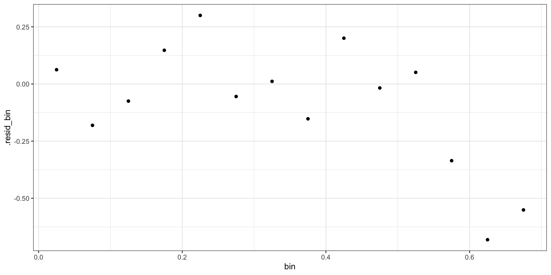
\[ r_i = \frac{Y_i - E(Y_i)}{\sqrt{Var(Y_i)}} = \frac{Y_i - \hat{p}_i}{\sqrt{\hat{p}_i(1-\hat{p}_i)}} \]
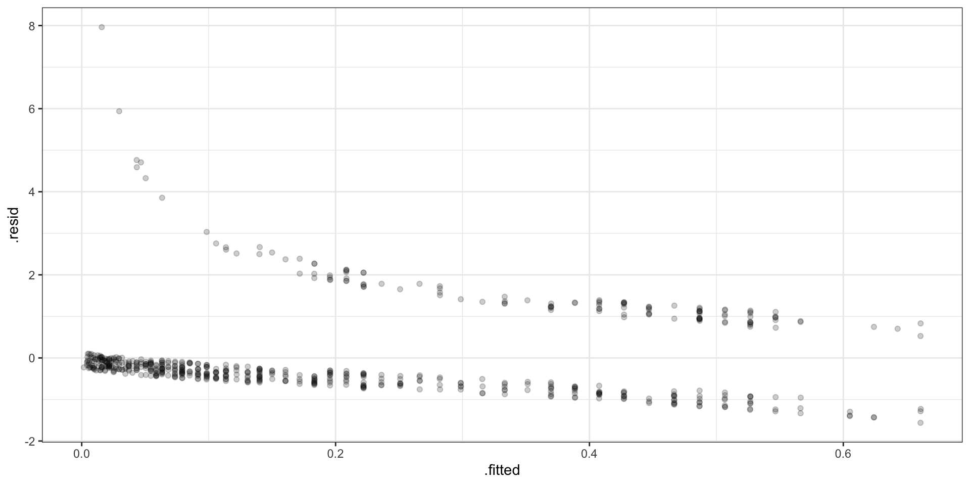
Binned Pearson Residuals
Deviance Residuals
\[ \begin{aligned} d_i = &\text{sign}(Y_i-\hat{p_i}) \, \times \\ &\sqrt{ -2 \left(Y_i \log \hat{p}_i+(1-Y_i)\log (1 - \hat{p}_i) \right) } \end{aligned} \]
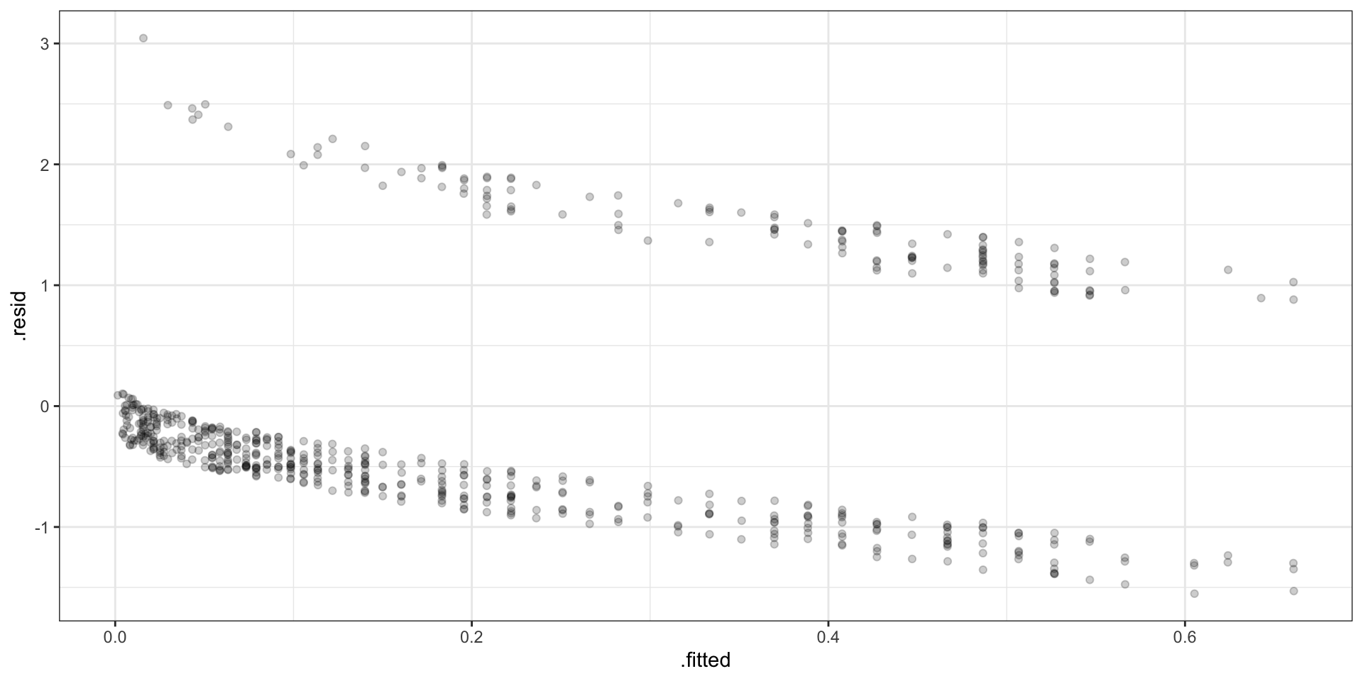
Binned Deviance Residuals
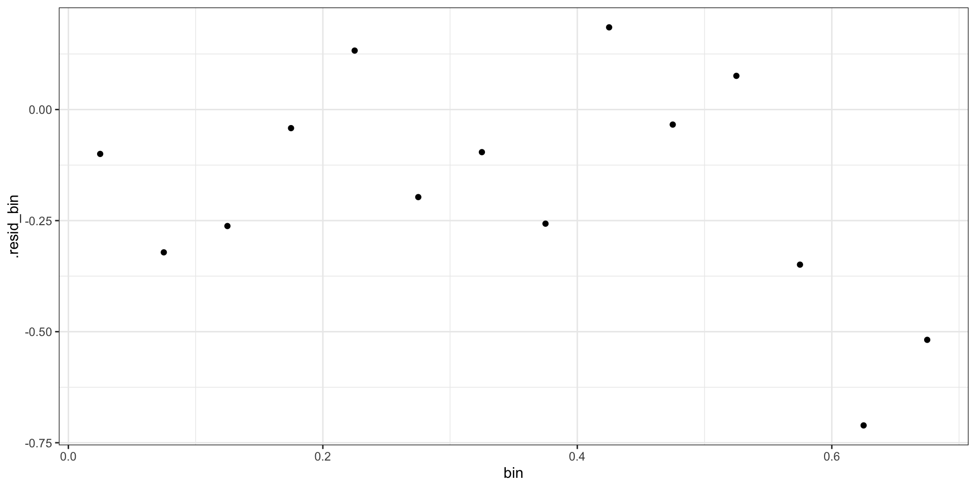
Checking Deviance
Call:  glm(formula = presence ~ SegSumT, family = binomial, data = anguilla_train)

Coefficients:
(Intercept)      SegSumT
   -15.0220       0.8005

Degrees of Freedom: 617 Total (i.e. Null);  616 Residual
Null Deviance:      627.8
Residual Deviance: 501.9 AIC: 505.9Sta 344 - Fall 2022
