Linear Models
Lecture 02
Dr. Colin Rundel
Linear Models Basics
Pretty much everything we a going to see in this course will fall under the umbrella of either linear or generalized linear models.
In previous classes most of your time has likely been spent with the simple iid case,
\[ y_i = \beta_0 + \beta_1 \, x_{i1} + \cdots + \beta_p \, x_{ip} + \epsilon_i \]
\[ \epsilon_i \overset{iid}{\sim} N(0, \sigma^2) \]
these models can also be expressed simply as,
\[ y_i \overset{iid}{\sim} N(\beta_0 + \beta_1 \, x_{i1} + \cdots + \beta_p \, x_{ip},~ \sigma^2) \]
Some notes on notation
Observed values and scalars will usually be lower case letters, e.g. \(x_i, y_i, z_{ij}\).
Parameters will usually be greek symbols, e.g. \(\mu, \sigma, \rho\).
Vectors and matrices will be shown in bold, e.g. \(\boldsymbol{\mu}, \boldsymbol{X}, \boldsymbol{\Sigma}\).
Elements of a matrix (or vector) will be referenced with {}s, e.g.\(\big\{ \boldsymbol{Y} \big\}_{i}, \big\{ \boldsymbol{\Sigma} \big\}_{ij}\)
Random variables will be indicated by ~, e.g. \(x \sim \text{Norm}(0,1), z \sim \text{Gamma}(1,1)\)
Matrix / vector transposes will be indicated with \('\), e.g. \(\boldsymbol{A}', (1-\boldsymbol{B})'\)
Linear model - matrix notation
We can also express a linear model using matrix notation as follows,
\[ \begin{aligned} \underset{n \times 1}{\boldsymbol{Y}} = \underset{n \times p}{\boldsymbol{X}} \, \underset{p \times 1}{\boldsymbol{\beta}} + \underset{n \times 1}{\boldsymbol{\epsilon}} \\ \underset{n \times 1}{\boldsymbol{\epsilon}} \sim N(\underset{n \times 1}{\boldsymbol{0}}, \; \sigma^2 \underset{n \times n}{\mathbb{1}_n}) \end{aligned} \]
or alternative as,
\[ \underset{n \times 1}{\boldsymbol{Y}} \sim N\left(\underset{n \times p}{\boldsymbol{X}} \, \underset{p \times 1}{\boldsymbol{\beta}},~ \sigma^2 \underset{n \times n}{\mathbb{1}_n}\right) \]
Multivariate Normal Distribution - Review
For an \(n\)-dimension multivate normal distribution with covariance \(\boldsymbol{\Sigma}\) (positive semidefinite) can be written as
\[ \underset{n \times 1}{\boldsymbol{Y}} \sim N(\underset{n \times 1}{\boldsymbol{\mu}}, \; \underset{n \times n}{\boldsymbol{\Sigma}}) \]
where \(\big\{\boldsymbol{\Sigma}\big\}_{ij} = \rho_{ij} \sigma_i \sigma_j\)
\[ \begin{pmatrix} y_1\\ y_2\\ \vdots\\ y_n \end{pmatrix} \sim N\left( \begin{pmatrix} \mu_1\\ \mu_2\\ \vdots\\ \mu_n \end{pmatrix}, \, \begin{pmatrix} \rho_{11}\sigma_1\sigma_1 & \rho_{12}\sigma_1\sigma_2 & \cdots & \rho_{1n}\sigma_1\sigma_n \\ \rho_{21}\sigma_2\sigma_1 & \rho_{22}\sigma_2\sigma_2 & \cdots & \rho_{2n}\sigma_2\sigma_n\\ \vdots & \vdots & \ddots & \vdots \\ \rho_{n1}\sigma_n\sigma_1 & \rho_{n2}\sigma_n\sigma_2 & \cdots & \rho_{nn}\sigma_n\sigma_n \\ \end{pmatrix} \right) \]
Multivariate Normal Distribution - Density
For the \(n\) dimensional multivate normal given on the last slide, its density is given by
\[ f\big(\boldsymbol{Y} | \boldsymbol{\mu}, \boldsymbol{\Sigma}\big) = (2\pi)^{-n/2} \; \det(\boldsymbol{\Sigma})^{-1/2} \; \exp{\left(-\frac{1}{2} \underset{1 \times n}{(\boldsymbol{Y}-\boldsymbol{\mu})'} \underset{n \times n}{\boldsymbol{\Sigma}^{-1}} \underset{n \times 1}{(\boldsymbol{Y}-\boldsymbol{\mu})}\right)} \]
and its log density is given by
\[ \log f\big(\boldsymbol{Y} | \boldsymbol{\mu}, \boldsymbol{\Sigma}\big) = -\frac{n}{2} \log 2\pi - \frac{1}{2} \log \det(\boldsymbol{\Sigma}) - \frac{1}{2} \underset{1 \times n}{(\boldsymbol{Y}-\boldsymbol{\mu})'} \underset{n \times n}{\boldsymbol{\Sigma}^{-1}} \underset{n \times 1}{(\boldsymbol{Y}-\boldsymbol{\mu})} \]
Some useful identities
The following come from the Matrix Cookbook Chapters 1 & 2.
\[ \begin{aligned} (\boldsymbol{A} \boldsymbol{B})' &= \boldsymbol{B}' \boldsymbol{A}' \\ (\boldsymbol{A} + \boldsymbol{B})' &= \boldsymbol{A}' + \boldsymbol{B}' \\ (\boldsymbol{A}')^{-1} &= (\boldsymbol{A}^{-1})' \\ (\boldsymbol{A}\boldsymbol{B}\boldsymbol{C}\ldots)^{-1} &= \ldots\boldsymbol{C}^{-1} \boldsymbol{B}^{-1} \boldsymbol{A}^{-1} \\ \\ \det(\boldsymbol{A}') &= \det(\boldsymbol{A}) \\ \det(\boldsymbol{A} \boldsymbol{B}) &= \det(\boldsymbol{A}) \det(\boldsymbol{B}) \\ \det(c\boldsymbol{A}) &= c^n \det(\boldsymbol{A}) \\ \det(\boldsymbol{A}^n) &= \det(\boldsymbol{A})^n \\ \end{aligned} \]
\[ \begin{aligned} \partial \boldsymbol{A} &= 0 \qquad\qquad \text{(where $\boldsymbol{A}$ is constant)}\\ \partial (a\boldsymbol{X}) &= a (\partial \boldsymbol{A})\\ \partial (\boldsymbol{X} + \boldsymbol{Y}) &= \partial \boldsymbol{X} + \partial \boldsymbol{Y} \\ \partial (\boldsymbol{X} \boldsymbol{Y}) &= (\partial \boldsymbol{X}) \boldsymbol{Y} + \boldsymbol{X} (\partial \boldsymbol{Y}) \\ \partial (\boldsymbol{X}') &= (\partial \boldsymbol{X})' \\ \partial (\boldsymbol{X}'\boldsymbol{A}\boldsymbol{X}) &= (\boldsymbol{A} + \boldsymbol{A}')\boldsymbol{X} \\ \end{aligned} \]
Maximum Likelihood - \(\boldsymbol{\beta}\) (iid)
Maximum Likelihood - \(\sigma^2\) (iid)
A Quick Example
Parameters -> Synthetic Data
Lets generate some simulated data where the underlying model is known and see how various regression procedures function.
\[ y_i = \beta_0 + \beta_1 x_{1i} + \beta_2 x_{2i} + \beta_3 x_{3i} +\epsilon_i \]
\[ \epsilon_i \sim N(0,1) \]
\[ \beta_0 = 0.7, \beta_1 = 1.5, \beta_2 = -2.2, \beta_3 = 0.1 \]
Model Matrix
# A tibble: 100 × 4
   `(Intercept)`      X1       X2      X3
           <dbl>   <dbl>    <dbl>   <dbl>
 1             1  0.557   0.897   -1.46
 2             1  0.758   0.375   -0.945
 3             1  0.273   3.81    -0.675
 4             1  1.41   -0.0745   0.514
 5             1  1.01    0.623   -1.99
 6             1  0.942  -0.00618  0.700
 7             1  1.66    1.57     0.0478
 8             1 -1.09    0.766    1.33
 9             1 -0.296   1.40    -0.0914
10             1 -0.0604  0.396   -0.0527
# … with 90 more rows
Pairs plot
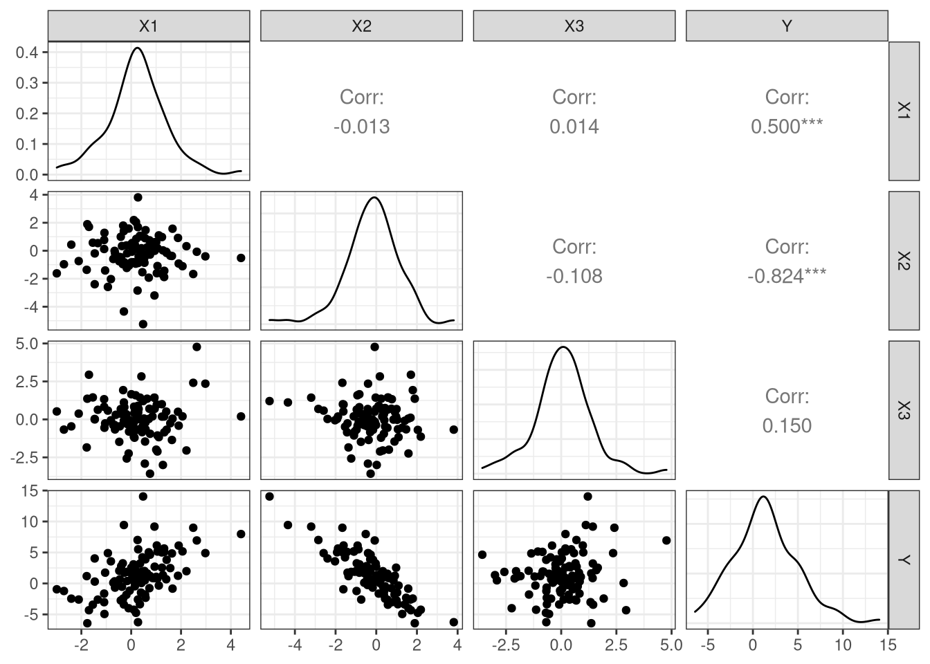
Least squares fit
Let \(\hat{\boldsymbol{Y}}\) be our estimate for \(\boldsymbol{Y}\) based on our estimate of \(\boldsymbol{\beta}\),
\[ \hat{\boldsymbol{Y}} = \hat{\beta}_0 + \hat{\beta}_1 \, \boldsymbol{X}_{1} + \hat{\beta}_2 \, \boldsymbol{X}_{2} + \hat{\beta}_3 \, \boldsymbol{X}_{3} = \boldsymbol{X}\, \hat{\boldsymbol{\beta}} \]
The least squares estimate, \(\hat{\boldsymbol{\beta}}_{ls}\), is given by
\[ \underset{\boldsymbol{\beta}}{\text{argmin}} \sum_{i=1}^n \left( Y_i - \boldsymbol{X}_{i\cdot} \boldsymbol{\beta} \right)^2 \]
Previously we showed that,
\[ \hat{\boldsymbol{\beta}}_{ls} = (\boldsymbol{X}' \boldsymbol{X})^{-1} \boldsymbol{X}' \, \boldsymbol{Y} \]
Beta estimate
                  [,1]
(Intercept)  0.5522298
X1           1.4708769
X2          -2.1761159
X3 0.1535830Bayesian regression model
Basics of Bayes
We will be fitting the same model as described above, we just need to provide some additional information in the form of a prior for our model parameters (the \(\beta\)s and \(\sigma^2\)).
\[ \begin{aligned} f(\theta | x) &= \frac{f(x | \theta) \; \pi(\theta)}{\int f(x|\theta) d\theta} \\ &\propto f(x|\theta) \; \pi(\theta) \end{aligned} \]
The posterior (\(f(\theta|x)\)) reflects an updated set of beliefs about the parameters (\(\theta\)) based on the observed data (\(x\)) via the likelihood (\(f(x|\theta)\))
Most of the time the posterior will not have a closed form so we will use a technique like MCMC to draw samples
Our inference will be based on the posterior distribution and not a point estimate (e.g. MLE)
brms
We will be using a package called brms for most of our Bayesian model fitting
it has a convenient model specification syntax
mostly sensible prior defaults
supports most of the model types we will be exploring
uses Stan behind the scenes
brms + linear regression
Running /usr/lib64/R/bin/R CMD SHLIB foo.c
gcc -m64 -I"/usr/include/R" -DNDEBUG   -I"/usr/lib64/R/library/Rcpp/include/"  -I"/usr/lib64/R/library/RcppEigen/include/"  -I"/usr/lib64/R/library/RcppEigen/include/unsupported"  -I"/usr/lib64/R/library/BH/include" -I"/usr/lib64/R/library/StanHeaders/include/src/"  -I"/usr/lib64/R/library/StanHeaders/include/"  -I"/usr/lib64/R/library/RcppParallel/include/"  -I"/usr/lib64/R/library/rstan/include" -DEIGEN_NO_DEBUG  -DBOOST_DISABLE_ASSERTS  -DBOOST_PENDING_INTEGER_LOG2_HPP  -DSTAN_THREADS  -DBOOST_NO_AUTO_PTR  -include '/usr/lib64/R/library/StanHeaders/include/stan/math/prim/mat/fun/Eigen.hpp'  -D_REENTRANT -DRCPP_PARALLEL_USE_TBB=1   -I/usr/local/include   -fpic  -O2  -fexceptions -g -grecord-gcc-switches -pipe -Wall -Werror=format-security -Wp,-D_FORTIFY_SOURCE=2 -Wp,-D_GLIBCXX_ASSERTIONS -specs=/usr/lib/rpm/redhat/redhat-hardened-cc1 -fstack-protector-strong -specs=/usr/lib/rpm/redhat/redhat-annobin-cc1  -m64  -mtune=generic -fasynchronous-unwind-tables -fstack-clash-protection -fcf-protection  -c foo.c -o foo.o
In file included from /usr/lib64/R/library/RcppEigen/include/Eigen/Dense:1,
                 from /usr/lib64/R/library/StanHeaders/include/stan/math/prim/mat/fun/Eigen.hpp:13,
                 from <command-line>:
/usr/lib64/R/library/RcppEigen/include/Eigen/Core:82:12: fatal error: new: No such file or directory
   82 |   #include <new>
      |            ^~~~~
compilation terminated.
make: *** [/usr/lib64/R/etc/Makeconf:168: foo.o] Error 1

SAMPLING FOR MODEL '63bfe1fe670faa5c207a7d2d657dea78' NOW (CHAIN 1).
Chain 1:
Chain 1: Gradient evaluation took 2e-05 seconds
Chain 1: 1000 transitions using 10 leapfrog steps per transition would take 0.2 seconds.
Chain 1: Adjust your expectations accordingly!
Chain 1:
Chain 1:
Chain 1: Iteration:    1 / 2000 [  0%]  (Warmup)
Chain 1: Iteration:  200 / 2000 [ 10%]  (Warmup)
Chain 1: Iteration:  400 / 2000 [ 20%]  (Warmup)
Chain 1: Iteration:  600 / 2000 [ 30%]  (Warmup)
Chain 1: Iteration:  800 / 2000 [ 40%]  (Warmup)
Chain 1: Iteration: 1000 / 2000 [ 50%]  (Warmup)
Chain 1: Iteration: 1001 / 2000 [ 50%]  (Sampling)
Chain 1: Iteration: 1200 / 2000 [ 60%]  (Sampling)
Chain 1: Iteration: 1400 / 2000 [ 70%]  (Sampling)
Chain 1: Iteration: 1600 / 2000 [ 80%]  (Sampling)
Chain 1: Iteration: 1800 / 2000 [ 90%]  (Sampling)
Chain 1: Iteration: 2000 / 2000 [100%]  (Sampling)
Chain 1:
Chain 1:  Elapsed Time: 0.025025 seconds (Warm-up)
Chain 1:                0.02603 seconds (Sampling)
Chain 1:                0.051055 seconds (Total)
Chain 1:

SAMPLING FOR MODEL '63bfe1fe670faa5c207a7d2d657dea78' NOW (CHAIN 2).
Chain 2:
Chain 2: Gradient evaluation took 7e-06 seconds
Chain 2: 1000 transitions using 10 leapfrog steps per transition would take 0.07 seconds.
Chain 2: Adjust your expectations accordingly!
Chain 2:
Chain 2:
Chain 2: Iteration:    1 / 2000 [  0%]  (Warmup)
Chain 2: Iteration:  200 / 2000 [ 10%]  (Warmup)
Chain 2: Iteration:  400 / 2000 [ 20%]  (Warmup)
Chain 2: Iteration:  600 / 2000 [ 30%]  (Warmup)
Chain 2: Iteration:  800 / 2000 [ 40%]  (Warmup)
Chain 2: Iteration: 1000 / 2000 [ 50%]  (Warmup)
Chain 2: Iteration: 1001 / 2000 [ 50%]  (Sampling)
Chain 2: Iteration: 1200 / 2000 [ 60%]  (Sampling)
Chain 2: Iteration: 1400 / 2000 [ 70%]  (Sampling)
Chain 2: Iteration: 1600 / 2000 [ 80%]  (Sampling)
Chain 2: Iteration: 1800 / 2000 [ 90%]  (Sampling)
Chain 2: Iteration: 2000 / 2000 [100%]  (Sampling)
Chain 2:
Chain 2:  Elapsed Time: 0.024312 seconds (Warm-up)
Chain 2:                0.024222 seconds (Sampling)
Chain 2:                0.048534 seconds (Total)
Chain 2:
Model results
 Family: gaussian
  Links: mu = identity; sigma = identity
Formula: Y ~ X1 + X2 + X3
   Data: d (Number of observations: 100)
  Draws: 2 chains, each with iter = 2000; warmup = 1000; thin = 1;
         total post-warmup draws = 2000

Population-Level Effects:
          Estimate Est.Error l-95% CI u-95% CI Rhat Bulk_ESS Tail_ESS
Intercept     0.55      0.11     0.35     0.76 1.00     2623     1609
X1            1.47      0.09     1.29     1.64 1.00     2292     1416
X2           -2.18      0.08    -2.33    -2.02 1.00     2294     1604
X3            0.15      0.08    -0.00     0.30 1.00     2403     1297

Family Specific Parameters:
      Estimate Est.Error l-95% CI u-95% CI Rhat Bulk_ESS Tail_ESS
sigma     1.03      0.08     0.89     1.20 1.00     2460     1420

Draws were sampled using sampling(NUTS). For each parameter, Bulk_ESS
and Tail_ESS are effective sample size measures, and Rhat is the potential
scale reduction factor on split chains (at convergence, Rhat = 1).
Model visual summary
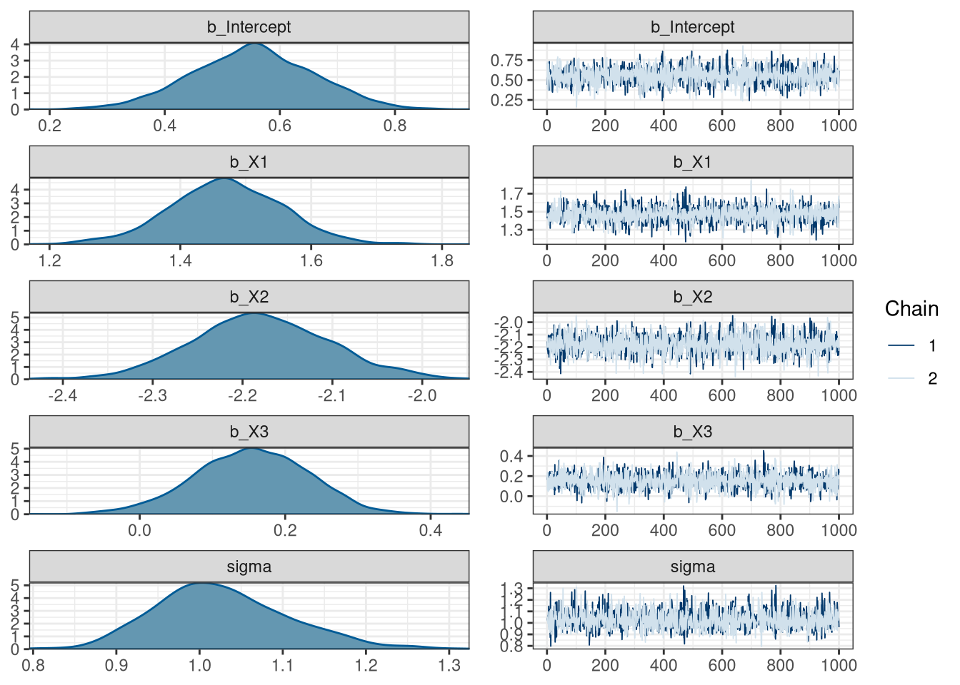
What about the priors?
tidybayes
# A tibble: 10,000 × 5
# Groups:   .variable [5]
   .chain .iteration .draw .variable   .value
    <int>      <int> <int> <chr>        <dbl>
 1      1          1     1 b_Intercept  0.440
 2      1          2     2 b_Intercept  0.524
 3      1          3     3 b_Intercept  0.544
 4      1          4     4 b_Intercept  0.502
 5      1          5     5 b_Intercept  0.567
 6      1          6     6 b_Intercept  0.569
 7      1          7     7 b_Intercept  0.373
 8      1          8     8 b_Intercept  0.731
 9      1          9     9 b_Intercept  0.379
10      1         10    10 b_Intercept  0.514
# … with 9,990 more rows
tidybayes + posterior summaries
(post_sum = post %>%
  group_by(.variable, .chain) %>%
  summarize(
    post_mean = mean(.value),
    post_median = median(.value)
  )
)
# A tibble: 10 × 4
# Groups: .variable [5]
.variable .chain post_mean post_median
<chr> <int> <dbl> <dbl>
1 b_Intercept 1 0.556 0.555
2 b_Intercept 2 0.550 0.553
3 b_X1 1 1.47 1.47
4 b_X1 2 1.47 1.47
5 b_X2 1 -2.18 -2.18
6 b_X2 2 -2.18 -2.18
7 b_X3 1 0.157 0.157
8 b_X3 2 0.151 0.152
9 sigma 1 1.03 1.02
10 sigma 2 1.02 1.02 tidybayes + ggplot - traceplot
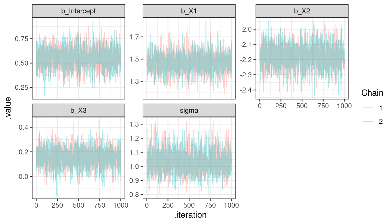
Tidy Bayes + ggplot - Density plot
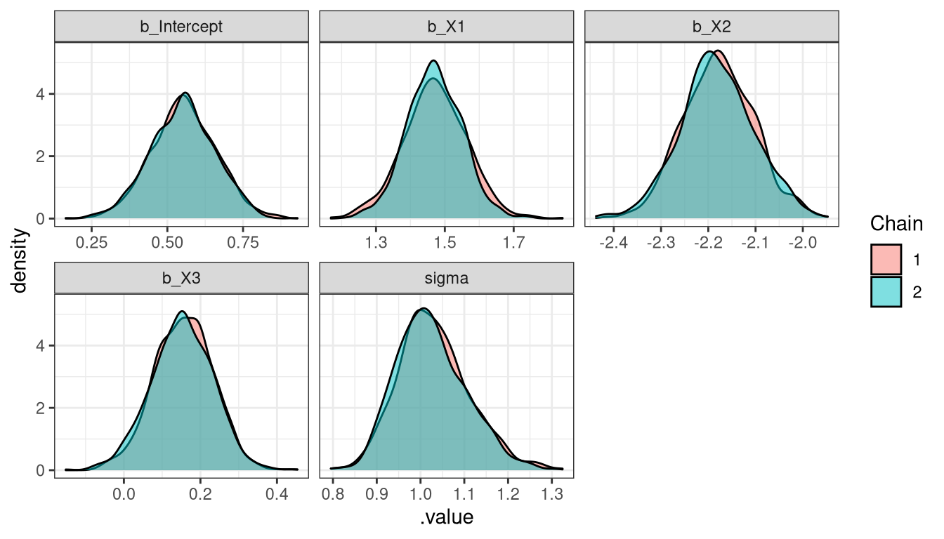
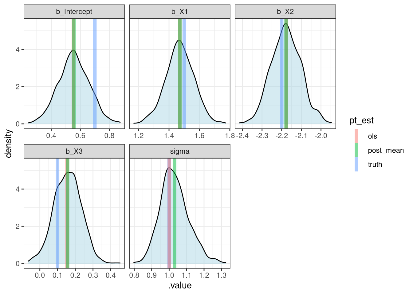
Comparing Approaches
(pt_est = post_sum %>%
  filter(.chain == 1) %>%
  ungroup() %>%
  mutate(
    truth = c(beta, sigma),
    ols   = c(l$coefficients, sd(l$residuals))
  ) %>%
  select(.variable, truth, ols, post_mean)
)
# A tibble: 5 × 4
.variable truth ols post_mean
<chr> <dbl> <dbl> <dbl>
1 b_Intercept 0.7 0.552 0.556
2 b_X1 1.5 1.47 1.47
3 b_X2 -2.2 -2.18 -2.18
4 b_X3 0.1 0.154 0.157
5 sigma 1 1.00 1.03 Comparing Approaches - code
post %>%
  filter(.chain == 1) %>%
  ggplot(aes(x=.value)) +
  geom_density(alpha=0.5, fill="lightblue") +
  facet_wrap(~.variable, scale="free_x") +
  geom_vline(
    data = pt_est %>% tidyr::pivot_longer(cols = truth:post_mean, names_to = "pt_est", values_to = "value"),
    aes(xintercept = value, color=pt_est),
    alpha = 0.5, size=2
  )
Comparing Approaches - plot
Sta 344 - Fall 2022